L2 Regularization: Parameters and Bias-Variance

Hello! Welcome back to our study of linear regression.

In our last lesson, we formulated the Ridge regression model and derived its closed-form solution: ${\hat{\mathbf{\beta }}}_{\text{Ridge}}=({\mathbf{X}}^T\mathbf{X}+\lambda \mathbf{I}{)}^{-1}{\mathbf{X}}^T\mathbf{y}$. We established that by adding the term $\lambda \mathbf{I}$, we ensure the matrix is always invertible, providing a stable and unique solution even in the presence of multicollinearity.

Today, we will analyze the profound consequences of adding this penalty term. Our learning outcome is to explain the effect of L2 regularization on model parameters and the bias-variance trade-off. We will dissect how Ridge regression alters the coefficient estimates and then dive into a rigorous mathematical analysis of its impact on the model's bias and variance, which are the fundamental components of prediction error.

1. The Shrinkage Effect on Model Parameters

The most immediate effect of the L2 penalty is that it shrinks the regression coefficients towards zero. To build a clear intuition for this, let's consider the special case of an orthonormal design matrix, where ${\mathbf{X}}^T\mathbf{X}=n\mathbf{I}$ (assuming features have been standardized to have mean 0 and standard deviation 1, which is common practice when using regularization).

In this scenario, the OLS solution simplifies to ${\hat{\mathbf{\beta }}}_{\text{OLS}}=(n\mathbf{I}{)}^{-1}{\mathbf{X}}^T\mathbf{y}=\frac{1}{n}{\mathbf{X}}^T\mathbf{y}$.
The Ridge solution becomes:

$${\hat{\mathbf{\beta }}}_{\text{Ridge}}=(n\mathbf{I}+\lambda \mathbf{I}{)}^{-1}{\mathbf{X}}^T\mathbf{y}=((n+\lambda )\mathbf{I}{)}^{-1}{\mathbf{X}}^T\mathbf{y}=\frac{1}{n+\lambda }{\mathbf{X}}^T\mathbf{y}$$

By substituting the OLS solution, we get a direct relationship:

$${\hat{\mathbf{\beta }}}_{\text{Ridge}}=\frac{n}{n+\lambda }\left(\frac{1}{n}{\mathbf{X}}^T\mathbf{y}\right)=\frac{n}{n+\lambda }{\hat{\mathbf{\beta }}}_{\text{OLS}}$$

This shows that the Ridge coefficients are a scaled-down version of the OLS coefficients. As $\lambda$ increases, the scaling factor $\frac{n}{n+\lambda }$ gets smaller, and the coefficients are shrunk more aggressively towards zero.

Geometric Interpretation

We can also visualize this effect. The OLS solution finds the coefficient vector $\mathbf{\beta }$ that minimizes the Residual Sum of Squares (RSS). This can be visualized as finding the center of a set of elliptical contours representing the RSS value. The Ridge penalty, $\lambda ||\mathbf{\beta }|{|}_2^2$, imposes a constraint: it prefers solutions where the squared L2-norm of $\mathbf{\beta }$ is small. This constraint region is a circle (in 2D) or a hypersphere centered at the origin.

The Ridge solution is found at the point of tangency between the RSS ellipse and the L2 constraint circle.

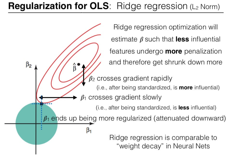
This geometric view shows that Ridge doesn't just shrink all coefficients equally. It applies a "budget" to the sum of squared coefficients. To stay within this budget, it disproportionately shrinks the coefficients of less influential features.

2. Decomposing the Error: The Bias-Variance Trade-off

We've established that Ridge regression produces estimates ${\hat{\mathbf{\beta }}}_{\text{Ridge}}$ that are different from ${\hat{\mathbf{\beta }}}_{\text{OLS}}$. Since the OLS estimator is unbiased (under the classical assumptions), it follows that the Ridge estimator must be biased. A biased estimator is one whose expected value is not equal to the true parameter value.

So, why would we ever prefer a biased estimator? The answer lies in the bias-variance trade-off. The total expected error of a model can be decomposed into three parts:

$$\text{Expected Prediction Error}={\text{Bias}}^2+\text{Variance}+\text{Irreducible Error}$$

• Bias: The error from erroneous assumptions in the learning algorithm. High bias can cause an algorithm to miss relevant relations between features and target outputs (underfitting).
• Variance: The error from sensitivity to small fluctuations in the training set. High variance can cause an algorithm to model the random noise in the training data (overfitting).
• Irreducible Error: Noise inherent in the problem itself.

Ridge regression works by introducing a small amount of bias in exchange for a significant reduction in variance. To prove this rigorously, we will derive the expressions for the bias and variance of the Ridge estimator.

The following resource provides a detailed, step-by-step derivation that aligns with your interest in mathematical depth. We will work through its main results.

The Bias of the Ridge Estimator

Let's summarize the derivation you just studied. We start by finding the expected value of the Ridge estimator, $\hat{\mathbf{w}}$ (using the notation from the paper, which is equivalent to our ${\hat{\mathbf{\beta }}}_{\text{Ridge}}$), assuming the true model is $\mathbf{y}={\mathbf{X}}^T{\mathbf{w}}^{\ast }+\mathbf{ϵ}$ with $E[\mathbf{ϵ}]=0$.

1. Expectation of the Estimator:

   $$E[\hat{\mathbf{w}}]=E[(\mathbf{X}{\mathbf{X}}^T+\lambda \mathbf{I}{)}^{-1}\mathbf{Xy}]=(\mathbf{X}{\mathbf{X}}^T+\lambda \mathbf{I}{)}^{-1}\mathbf{X}E[\mathbf{y}]$$

   Since $E[\mathbf{y}]={\mathbf{X}}^T{\mathbf{w}}^{\ast }$, we get:

   $$E[\hat{\mathbf{w}}]=(\mathbf{X}{\mathbf{X}}^T+\lambda \mathbf{I}{)}^{-1}\mathbf{X}{\mathbf{X}}^T{\mathbf{w}}^{\ast }$$

2. Bias Calculation:
   The bias of the estimator is $\text{Bias}(\hat{\mathbf{w}})=E[\hat{\mathbf{w}}]-{\mathbf{w}}^{\ast }$. A clever algebraic trick shown in the paper reveals:

   $$E[\hat{\mathbf{w}}]={\mathbf{w}}^{\ast }-\lambda (\mathbf{X}{\mathbf{X}}^T+\lambda \mathbf{I}{)}^{-1}{\mathbf{w}}^{\ast }$$

   Thus, the bias is:

   $$\text{Bias}(\hat{\mathbf{w}})=-\lambda (\mathbf{X}{\mathbf{X}}^T+\lambda \mathbf{I}{)}^{-1}{\mathbf{w}}^{\ast }$$

   This is a crucial result. If $\lambda =0$, the bias is zero (recovering the unbiased OLS case). If $\lambda >0$, the estimator is biased, and the bias depends on the true parameters ${\mathbf{w}}^{\ast }$.

3. Behavior of Bias:
   The paper goes on to show that the squared bias of the predictions, summed over the training data, is a monotonically increasing function of $\lambda$. It starts at 0 for $\lambda =0$ and increases as we penalize the coefficients more heavily.

The Variance of the Ridge Estimator

Next, let's look at the variance. The variance measures how much the estimate $\hat{\mathbf{w}}$ would vary if we were to re-run the estimation on different training datasets (with different noise $\mathbf{ϵ}$).

1. Deviation from the Mean:
   The derivation starts from the difference between the estimator and its mean:

   $$\hat{\mathbf{w}}-E[\hat{\mathbf{w}}]=-(\mathbf{X}{\mathbf{X}}^T+\lambda \mathbf{I}{)}^{-1}\mathbf{X}\mathbf{ϵ}$$

   This shows that the variance comes entirely from the model's reaction to the noise $\mathbf{ϵ}$ in the data.

2. Variance Calculation:
   Using matrix trace properties and the assumption that the noise terms are independent with unit variance ($E[\mathbf{ϵ}{\mathbf{ϵ}}^T]={\sigma }^2\mathbf{I}$, where the paper assumes ${\sigma }^2=1$), the variance of the predictions is derived. Using the eigendecomposition of $\mathbf{X}{\mathbf{X}}^T=\mathbf{U}\mathbf{\Sigma }{\mathbf{U}}^T$, where ${\sigma }_i$ are the diagonal entries of $\mathbf{\Sigma }$ (eigenvalues), the variance simplifies to:

   $$\text{Var}={\sigma }^2\sum _{i=1}^d\frac{{\sigma }_i^2}{({\sigma }_i+\lambda {)}^2}$$

   (Note: The resource sets ${\sigma }^2=1$, but I've included it for generality).

3. Behavior of Variance:
   From this final form, we can see that the variance is a monotonically decreasing function of $\lambda$.

   • When $\lambda =0$, the variance is ${\sigma }^2\sum \frac{{\sigma }_i^2}{{\sigma }_i^2}={\sigma }^{2}d$, corresponding to the OLS variance.
   • As $\lambda \to \infty$, each term $\frac{{\sigma }_i^2}{({\sigma }_i+\lambda {)}^2}\to 0$, so the total variance approaches zero. This makes intuitive sense: a model that predicts zero regardless of the data has zero variance.

Test your understanding!

Based on the derivations, explain intuitively why the bias term depends on the true parameters ${\mathbf{w}}^{\ast }$, while the variance term depends on the noise variance ${\sigma }^2$.

Show answer

• Bias is a measure of how far the average estimate is from the true value. The shrinkage effect systematically pulls the estimates away from the true values ${\mathbf{w}}^{\ast }$ towards zero. The magnitude of this pull and the resulting error naturally depend on where the true values were to begin with. If ${\mathbf{w}}^{\ast }$ is already close to zero, the bias will be small. If ${\mathbf{w}}^{\ast }$ is large, the same shrinkage will introduce a larger bias.

• Variance is a measure of the estimator's sensitivity to the random noise in the specific training sample. It measures the spread of estimates around their own average, not around the true value. This spread is caused by the estimator fitting to the random noise $\mathbf{ϵ}$. Therefore, the variance formula fundamentally depends on the magnitude of that noise (${\sigma }^2$) and the structure of the data ($\mathbf{X}$), but not on the true parameters ${\mathbf{w}}^{\ast }$.

3. The Optimal Trade-off

We have established that as $\lambda$ increases:

• Bias² increases from 0.
• Variance decreases towards 0.

Since the total error is the sum of these opposing forces, there must be a "sweet spot"—an optimal value of $\lambda$ that minimizes the total error. This is the essence of the bias-variance trade-off.

This trade-off leads to a powerful and somewhat surprising theoretical result.

As you just read, the theorem states: There always exists a value $\lambda >0$ such that the Mean Squared Error (MSE) of the Ridge estimator is less than the MSE of the OLS estimator.

This guarantees that it is always possible to improve upon the OLS solution (in terms of expected prediction error) by introducing some bias through shrinkage. In practice, the optimal $\lambda$ is an unknown hyperparameter that we must estimate, typically using a method like cross-validation.

Conclusion

In this lesson, we have moved from deriving the Ridge estimator to rigorously analyzing its behavior. We have seen that the L2 penalty has a profound impact on both the model parameters and its statistical properties.

Key Takeaways:

• L2 regularization's primary effect on parameters is shrinkage: it pulls coefficient estimates towards zero, with a larger effect on less influential features.
• This shrinkage introduces bias into the estimator, as the expected value of the Ridge coefficients is no longer equal to the true parameter values.
• In return, shrinkage dramatically reduces the estimator's variance, making it less sensitive to the noise in the training data.
• This dynamic creates the bias-variance trade-off. By accepting a small amount of bias, we can achieve a larger reduction in variance, leading to a model with a lower overall Mean Squared Error.
• Theoretically, there is always a regularization strength $\lambda >0$ that yields a better predictive model than OLS ($\lambda =0$).

Preview of the Next Module:
We have now completed our deep dive into linear regression, covering its formulation, analytical solutions (OLS and Ridge), and statistical properties. This foundational knowledge of linear models is essential. We will now pivot from regression to a new task: classification. In the next module, we will begin our study of Logistic Regression, exploring how the principles of linear models can be adapted to predict categorical outcomes.