Defining Binary Classification

Hello! Welcome to the first lesson in our new module on classification.

In our previous module, we completed a thorough investigation of linear regression. We learned how to model problems where the goal is to predict a continuous numerical value, derived the OLS and Ridge regression solutions, and analyzed their statistical properties like bias and variance.

Today, we shift our focus from regression to classification. This is a vast and fundamental area of machine learning concerned with predicting discrete, categorical labels rather than continuous quantities. Our learning outcome for this lesson is to formulate the binary classification problem mathematically. We will define the components of the problem, establish the notation we'll use throughout this module, and understand why the methods we learned for regression are not directly suitable for this new task.

1. What is Classification?

In regression, we predict a quantity (e.g., house price, temperature). In classification, we predict a category (e.g., spam/not spam, malignant/benign tumor, fraudulent/valid transaction). The simplest and most common type of classification is binary classification, where there are only two possible outcome categories.

Let's begin by watching a short introduction from Professor Trevor Hastie, one of the authors of the seminal textbook "The Elements of Statistical Learning," who will contrast classification with regression.

As the video explains, the goal is to build a function, a classifier, that takes a feature vector $\mathbf{x}$ as input and outputs a predicted class label.

2. Can We Use Linear Regression for Classification?

A natural first question, given our extensive study of linear regression, is whether we can adapt it for classification. For a binary problem, we could encode the two labels as 0 and 1. For example, y = 0 for "benign" and y = 1 for "malignant". We could then perform a linear regression of y on our features X. To make a prediction, we could check if the predicted value $\hat{y}={\mathbf{x}}^T\mathbf{\beta }$ is greater than a threshold, like 0.5.

While this seems plausible, it introduces significant problems. The following video clips explain why this approach is flawed.

The key takeaways are:

1. Meaningless Predictions: A linear model ${\mathbf{x}}^T\mathbf{\beta }$ can produce any real number, but for a binary (0/1) problem, we are trying to model something that should behave like a probability. A predicted "probability" of 1.3 or -0.2 is nonsensical.
2. Artificial Ordering (in multi-class cases): If we have three classes (e.g., "stroke," "overdose," "seizure") and code them as 1, 2, and 3, linear regression would incorrectly assume that the "distance" between stroke and overdose is the same as the distance between overdose and seizure.

These issues make it clear that we need a different mathematical framework, one designed specifically for modeling categorical outcomes.

3. The Formal Mathematical Formulation

Let's now build the precise mathematical formulation for binary classification, which will serve as the foundation for the rest of this module. Your background in mathematics and programming will be helpful here as we define the data structures and objectives formally.

We will base our formulation on the definitions provided in the lecture notes from MIT's "Mathematics of Machine Learning" course.

Let's synthesize and expand on the key definitions from the reading.

• Data: We assume we have a dataset of $n$ independent and identically distributed (i.i.d.) observations: $$\mathcal{D}=\{({\mathbf{x}}^{(1)},y^{(1)}),({\mathbf{x}}^{(2)},y^{(2)}),\dots ,({\mathbf{x}}^{(n)},y^{(n)})\}$$
• Feature Space ($\mathcal{X}$): Each input ${\mathbf{x}}^{(i)}$ is a feature vector, which is an element of the feature space $\mathcal{X}$. In most ML applications, this is a $d$-dimensional Euclidean space, so $\mathcal{X}={\mathbb{R}}^d$.
• Label Space ($\{0,1\}$): Each output $y^{(i)}$ is a label. For binary classification, the label space consists of just two values, which by convention we denote as $\{0,1\}$.
• Classifier ($h$): The goal is to learn a function, called a classifier or hypothesis, that maps the feature space to the label space: $$h:\mathcal{X}\to \{0,1\}$$ This function takes a new, unseen feature vector $\mathbf{x}$ and predicts its label, $\hat{y}=h(\mathbf{x})$.

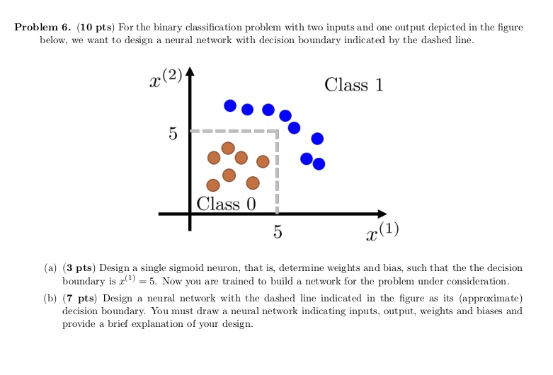
Visually, you can think of a classifier as creating a decision boundary in the feature space that separates the data points of one class from those of the other.

4. A Probabilistic Approach

Simply predicting a label (0 or 1) is useful, but often it's more valuable to know the model's confidence in its prediction. For instance, in medical diagnosis, knowing a tumor has a 98% probability of being malignant is more informative than just a "malignant" label, as it suggests a higher urgency than a 51% probability.

This leads to a more nuanced and powerful formulation of the classification problem: instead of learning a direct mapping to $\{0,1\}$, we aim to model the conditional probability that the label is 1, given the features.

As defined in the MIT notes, we introduce the regression function $\eta (\mathbf{x})$:

This expression is the cornerstone of probabilistic classification. It states that for a given feature vector $\mathbf{x}$, there is a specific probability that the corresponding label $Y$ is 1.

Under this view, the label $Y$ itself is a random variable that follows a Bernoulli distribution, with its parameter given by $\eta (\mathbf{x})$.

This is a precise mathematical statement of our assumption about the data-generating process. It elegantly captures the idea that even for the exact same features $\mathbf{x}$, the outcome might not be deterministic due to inherent randomness or unobserved factors (this is what the notes refer to as "noise").

Our objective now shifts from learning the classifier $h:\mathcal{X}\to \{0,1\}$ directly to learning the probability function $\eta :\mathcal{X}\to [0,1]$. If we can find a good approximation of $\eta (\mathbf{x})$, we can easily create a classifier by applying a threshold. The standard choice is 0.5:

Conclusion

In this lesson, we have formally defined the binary classification task, distinguishing it from the regression problems we studied previously. We established the precise mathematical language and notation required for a rigorous analysis.

Key Takeaways:

• Classification vs. Regression: Classification predicts a discrete category, while regression predicts a continuous value.
• Failure of Linear Regression: Applying linear regression to a 0/1 coded classification problem is flawed because it can produce predictions outside the meaningful [0, 1] range and doesn't naturally handle the probabilistic nature of class labels.
• Formal Formulation: A binary classification problem involves learning a classifier $h:{\mathbb{R}}^d\to \{0,1\}$ from a dataset of feature-label pairs $({\mathbf{x}}^{(i)},y^{(i)})$.
• Probabilistic View: A more powerful approach is to model the conditional probability $P(Y=1|X=\mathbf{x})$. This reframes the learning problem as finding a function that maps features to a probability in the interval $[0,1]$.

Preview of the Next Lesson:
We have established that our goal is to model the probability $P(Y=1|\mathbf{x})$. We need a function that takes our familiar linear combination of features, ${\mathbf{x}}^T\mathbf{\beta }$, which can produce any real number, and maps it to the $[0,1]$ interval required for a probability. In the next lesson, we will derive the logistic (sigmoid) function and explore its properties, showing why it is the perfect candidate for this task.