Understanding Speculative Decoding

Welcome to the next lesson in our module on inference performance optimization. In the previous lessons, we've tackled memory constraints by quantizing models and revolutionized KV cache management with PagedAttention. These optimizations are critical, but they still operate within the fundamental constraint of autoregressive generation: producing tokens one by one.

Today, we'll challenge that sequential process directly. This lesson introduces speculative decoding, an ingenious technique that allows a large language model to generate multiple tokens in a single step, significantly reducing latency. You will learn the core mechanism behind this method, where a small, fast "draft" model proposes candidate tokens that a larger, more accurate "target" model then verifies.

Your background in systems engineering gives you a unique perspective here. Speculative decoding is conceptually similar to speculative execution in CPUs, where a processor performs work before it's certain it's needed. Here, we're applying a similar "guess and check" philosophy to accelerate LLM inference.

1. The Problem: The Slow March of Single Tokens

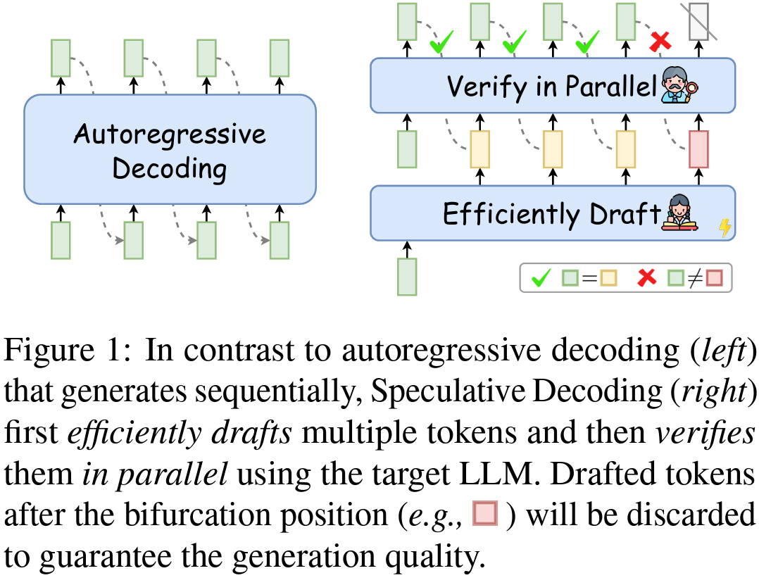
As we've established, standard autoregressive generation is a sequential process. To generate 100 tokens, the model must perform 100 separate forward passes. Each pass is memory-bound, limited by the speed at which the model's weights can be loaded from GPU HBM to the compute cores. This is the fundamental bottleneck that causes high latency.

Speculative decoding changes the game by moving from a one-token-at-a-time process to a speculate-then-verify loop.

2. The Core Idea: The Scientist and the Assistant

The most intuitive way to understand speculative decoding is through an analogy. Imagine your main, powerful LLM (the target model) is a meticulous, world-class scientist. The scientist is brilliant but slow and expensive. Now, imagine you hire a fast, energetic-but-less-experienced assistant (the draft model).

Instead of the scientist doing every routine step, the process looks like this:

1. The assistant quickly drafts a few steps of the experiment's results.
2. The scientist takes the draft and, in a single, efficient review, checks all the steps at once.
3. The scientist accepts all the correct steps, stops at the first mistake, corrects it, and hands the corrected work back to the assistant to continue drafting from there.

This way, the scientist's valuable time is spent verifying chunks of work, not performing every single step. This is precisely how speculative decoding works. A small, fast draft model generates a "draft" of the next few tokens, and the large, accurate target model verifies them in one efficient, parallel pass.

This video from Julien Simon gives a great high-level intuition for this process.

3. The Mechanism: A Three-Step Process

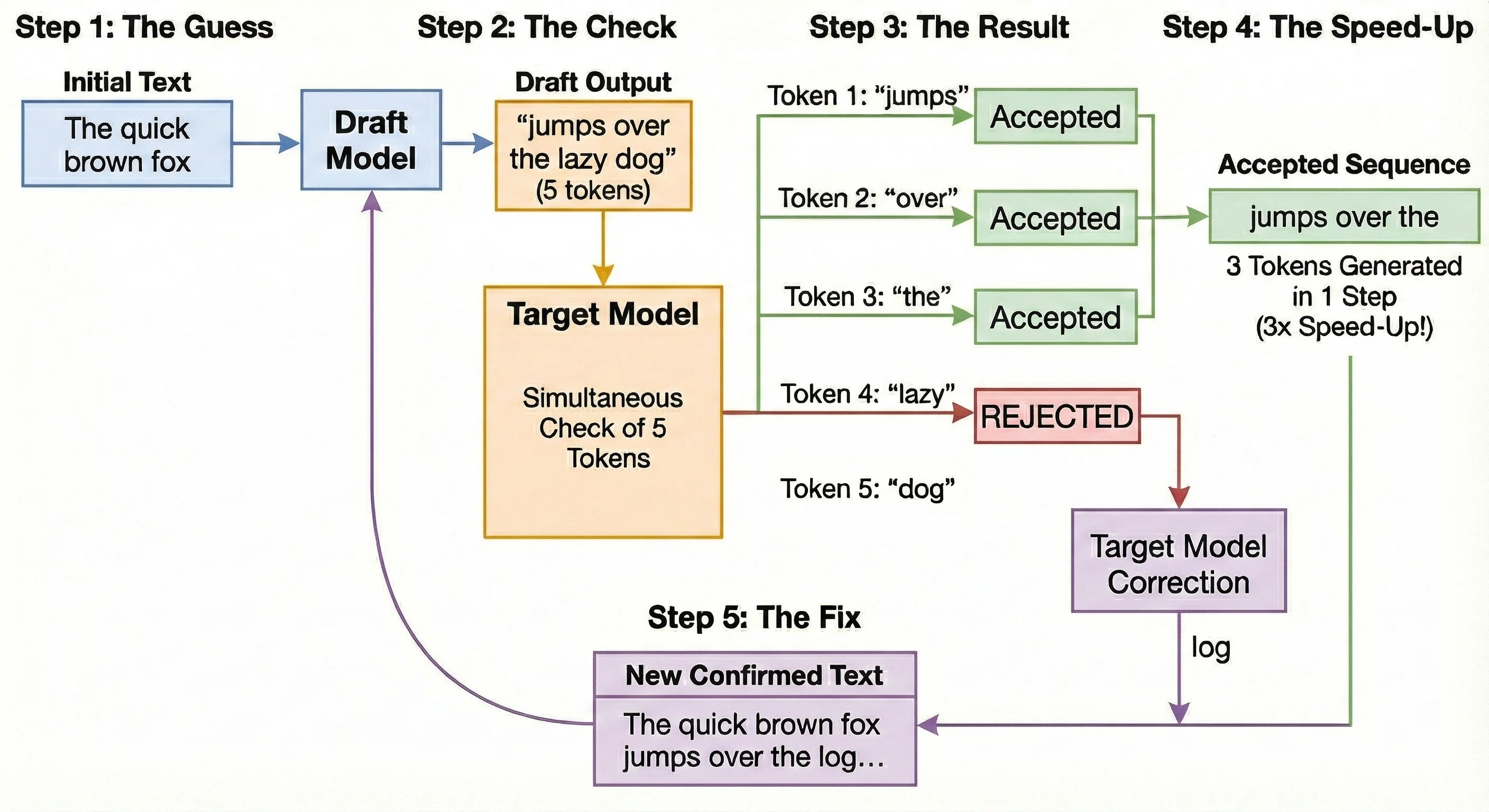
The speculative decoding workflow can be broken down into three key steps: Draft, Verify, and Accept/Reject.

Let's dive into the details of this process. The following video provides one of the clearest explanations of the underlying algorithm. We will walk through it step-by-step.

Let's break down those steps with a bit more detail.

Step 1: Draft Generation

The process begins with the small draft model. Given the current sequence, it autoregressively generates a short chain of K candidate tokens (e.g., K=5). This is fast because the draft model is small (e.g., 1B parameters vs. 7B for the target).

Step 2: Parallel Verification

This is where the magic happens. The target model receives the original sequence plus the K draft tokens. It then performs a single forward pass. Because of the parallel nature of the Transformer architecture, this one pass yields the probability distributions for the next token at every position along the sequence. We get K+1 probability distributions from the target model for the cost of just one run.

Step 3: Rejection Sampling

Now, we must decide which draft tokens to keep. We can't just trust the draft model; the final output must be identical to what the target model would have generated on its own. This guarantee is achieved with a clever probabilistic check called rejection sampling.

We iterate through the draft tokens one by one, comparing the probability the target model assigned to it, $q(x_i)$, with the probability the draft model assigned, $p(x_i)$.

For each token $x_i$ in the draft:

1. If $q(x_i)\ge p(x_i)$: The target model is at least as confident as the draft model, or more so. The token is accepted.
2. If $q(x_i)<p(x_i)$: The target model is less confident. We "roll a die" and accept the token with a probability of $\frac{q(x_i)}{p(x_i)}$. This corrects for the draft model's overconfidence.

This process continues until the first token is rejected. At that point, we discard that token and all subsequent draft tokens. We then sample a new, corrected token from an adjusted probability distribution derived from the target model. This ensures that even in a rejection case, we always generate at least one valid token.

The crucial outcome is that the distribution of tokens generated by this complex procedure is mathematically identical to the distribution of the target model alone. We get the speed-up without any loss in accuracy.

4. Why Is It Faster?

The performance gain comes from the number of tokens accepted in each round.

• Best Case: If all K draft tokens are accepted, we also get to sample one more token from the target model's final probability distribution. We generate K+1 tokens for the cost of one slow target model pass and K fast draft model passes.
• Worst Case: If the very first draft token is rejected, we discard the whole draft, sample one corrected token from the target model, and start over. In this scenario, the performance is roughly equivalent to standard autoregressive decoding (plus a small overhead from the draft run).

The actual speedup, typically 2-3x, depends on the acceptance rate—how often the draft model's predictions align with the target model's. This works especially well for "easy" parts of text generation (like common phrases or boilerplate code) where a smaller model can predict well.

5. Variations on the "Draft" Mechanism

A natural question is: where does the draft model come from? While the classic approach uses a smaller pre-trained model, other clever variations exist.

These variations all share the same principle: use a faster, cheaper mechanism to generate candidates that the main model can verify in parallel.

Conclusion

In this lesson, you've learned the fundamental mechanism of speculative decoding, a powerful technique for accelerating LLM inference by breaking the one-token-at-a-time bottleneck.

Here are the key takeaways:

• Core Problem: Standard autoregressive generation is slow because it's sequential and memory-bound.
• The Mechanism: Speculative decoding uses a small, fast draft model to generate a sequence of candidate tokens. The large, accurate target model then verifies all these candidates in a single, parallel forward pass.
• The Guarantee: A rejection sampling algorithm ensures that the final output distribution is mathematically identical to what the target model would have produced alone, meaning there is no loss of quality.
• The Result: Instead of one token per target model pass, you can generate multiple tokens, leading to significant latency reduction and throughput improvement.

You now understand the "how" and "why" behind this optimization. In our next lesson, we'll move to the practical application: you will configure speculative decoding in a serving framework and benchmark its impact on generation speed.