Vectorized Returns, Rolling Statistics, and Lagged Features

Hello. In the last lesson, you built a clean multi-stock price panel whose key is (symbol, date). That structure is exactly what prevents a return for INFY from accidentally using RELIANCE’s previous close—a small coding mistake with very large research consequences.

This lesson turns that panel into feature-ready research data. You will calculate per-stock returns, lags, moving averages, rolling volatility, and an exponentially weighted average using pandas and NumPy operations that scale across an entire universe. The central discipline is alignment: each value must be calculated from the intended earlier observations and made available only when those observations could actually have been known.

Study time: about 40 minutes.

---

Start with a sorted, per-symbol time series

Assume prices is the daily OHLCV panel from the preceding lesson, indexed by ("symbol", "date") and sorted:

import numpy as np
import pandas as pd

prices = prices.sort_index()

close = prices["close"].astype("float64")
close.index.names
# ["symbol", "date"]

Every calculation in this lesson must operate within each symbol. A plain .shift() or .pct_change() on the full long panel is unsafe: consecutive rows in the table can belong to different stocks.

For example, imagine this ordering:

symbol	date	close
INFY	2024-01-02	1514
INFY	2024-01-03	1528
RELIANCE	2024-01-02	2472
RELIANCE	2024-01-03	2483

A simple shift over the entire table happens to work only because it is sorted symbol-first. But at the boundary between INFY and RELIANCE, it would place INFY’s final close beside RELIANCE’s first close. Grouping makes the intended meaning explicit and remains correct even when the universe changes.

by_symbol = close.groupby(level="symbol", sort=False)

Think of by_symbol as an instruction to pandas: “perform this time-series calculation independently for each stock.”

Before proceeding, inspect the core assumptions:

assert prices.index.is_unique
assert prices.index.is_monotonic_increasing
assert close.notna().all()

The final assertion is deliberately strict for this introductory workflow. Later, the historical-data pipeline will distinguish genuine missing sessions from bad prices, suspensions, and data outages. For now, do not silently invent prices with forward-filling.

---

Returns: turn prices into comparable movements

Prices are not directly comparable across stocks. A ₹20 move is economically very different for a ₹100 stock than for a ₹2,500 stock. Returns express the move relative to the prior price.

The one-session arithmetic return is:

$$r_t=\frac{P_t}{P_{t-1}}-1$$

If a close rises from ₹100 to ₹103, the return is $0.03$, or 3%. If it falls from ₹100 to ₹97, the return is $-0.03$, or -3%.

The pandas method .pct_change() computes this fractional change. Despite its name, it does not multiply by 100.

Compute daily returns per stock:

features = pd.DataFrame(index=prices.index)

features["ret_1d"] = by_symbol.pct_change(fill_method=None)

The first observation for every stock is NaN, not zero. There is no prior close from which to calculate a return. Treating it as zero would claim the price was unchanged before the stock entered the dataset.

A five-session return can be calculated directly:

features["ret_5d"] = close / by_symbol.shift(5) - 1

Here, 5 means five observed bars for that symbol, not five calendar days. A daily dataset should ordinarily contain only exchange sessions, so holidays and weekends are absent rather than represented by zero-return rows.

Log returns

Log returns are often useful because they add across time:

$${\ell }_t=\log \left(\frac{P_t}{P_{t-1}}\right)$$

features["log_ret_1d"] = np.log(close / by_symbol.shift(1))

For ordinary daily equity moves, arithmetic and log returns are close, but they are not identical. A 10% gain followed by a 10% loss does not return to the starting price:

$$(1.10)(0.90)-1=-0.01$$

Log returns capture compounding through summation:

$$\log \left(\frac{P_t}{P_{t-k}}\right)=\sum _{j=0}^{k-1}{\ell }_{t-j}$$

For most swing-strategy rules, arithmetic returns are intuitive and sufficient. Log returns become especially convenient for statistical analysis and aggregating across holding periods.

---

Lags are an alignment tool, not just a convenience

A lag places an earlier value beside the current row. For a daily series, shift(1) means “the immediately preceding observed bar for this stock.”

features["close_lag_1"] = by_symbol.shift(1)
features["close_lag_5"] = by_symbol.shift(5)

At the row for 2024-01-10, close_lag_1 contains the close from the previous session; it does not change the date index itself.

Avoid shift(freq=...) here. A frequency shift changes timestamps, which can be useful in calendar work but is not what you want when creating a prior-bar feature. You want today’s row to retain today’s session label while holding information from an earlier session.

A standard momentum feature is simply a return over a longer lookback:

features["momentum_20d"] = close / by_symbol.shift(20) - 1

For a row dated Tuesday, this is known after Tuesday’s close because it includes Tuesday’s close. It can therefore support a decision placed after Tuesday’s close for execution on a later session. It cannot support a decision supposedly made before Tuesday’s session started.

That distinction becomes essential in backtesting.

---

Rolling statistics: summarize the recent past

A rolling window evaluates a statistic over a fixed number of preceding observations. A 20-session simple moving average at time $t$ is:

$${\text{SMA}}_{20,t}=\frac{1}{20}\sum _{i=0}^{19}{P}_{t-i}$$

It includes the current close and the 19 preceding closes.

features["sma_20"] = (
    close
    .groupby(level="symbol", sort=False)
    .rolling(window=20, min_periods=20)
    .mean()
    .droplevel(0)
    .reindex(prices.index)
)

The extra .droplevel(0) removes the grouping level that pandas adds to the rolling result. The .reindex(prices.index) makes the original panel order explicit before assigning the result.

A moving average smooths day-to-day noise. It is not a forecast by itself. It is a descriptive feature that can become part of a falsifiable rule later, such as comparing yesterday’s close with yesterday’s 20-day average.

The same rolling operation can estimate recent historical volatility. First calculate daily returns, then calculate their rolling standard deviation:

rolling_vol_20 = (
    features["ret_1d"]
    .groupby(level="symbol", sort=False)
    .rolling(window=20, min_periods=20)
    .std()
    .droplevel(0)
    .reindex(prices.index)
)

features["vol_20d"] = rolling_vol_20
features["vol_20d_annualized"] = rolling_vol_20 * np.sqrt(252.0)

vol_20d is the standard deviation of daily arithmetic returns over the past 20 observations. vol_20d_annualized applies the common square-root-of-time approximation using 252 trading sessions per year. Treat annualization as a convention for comparing risk estimates, not as a promise that future volatility will behave proportionally.

Using min_periods=20 means the statistic remains missing until there are 20 valid observations. This is generally preferable to allowing a two-day volatility estimate to masquerade as a 20-day estimate.

A few useful rolling calculations follow the same pattern:

Feature	pandas aggregation	Typical interpretation
Moving average	.rolling(20).mean()	Recent price level
Rolling standard deviation	.rolling(20).std()	Recent return variability
Rolling maximum	.rolling(20).max()	Highest recent price
Rolling minimum	.rolling(20).min()	Lowest recent price
Rolling mean volume	.rolling(20).mean() on volume	Recent liquidity proxy

The key point is that these operate on a window of observations for one stock, not on a window spanning whichever rows happen to be adjacent in the DataFrame.

---

Simple moving averages versus exponentially weighted averages

A simple moving average gives equal weight to every observation in its window. An exponentially weighted moving average, or EMA, gives more weight to recent prices and gradually less weight to older ones.

With span $s$, pandas uses a smoothing coefficient:

$$\alpha =\frac{2}{s+1}$$

The recursive form is:

$${\text{EMA}}_t=\alpha P_t+(1-\alpha ){\text{EMA}}_{t-1}$$

A 20-period EMA can be calculated for every symbol without a Python loop:

features["ema_20"] = (
    close
    .groupby(level="symbol", sort=False)
    .ewm(span=20, adjust=False, min_periods=20)
    .mean()
    .droplevel(0)
    .reindex(prices.index)
)

adjust=False uses the recursive formulation above, which is common in trading implementations. min_periods=20 maintains a consistent warm-up policy: do not treat the earliest, initialization-sensitive EMA values as fully established features.

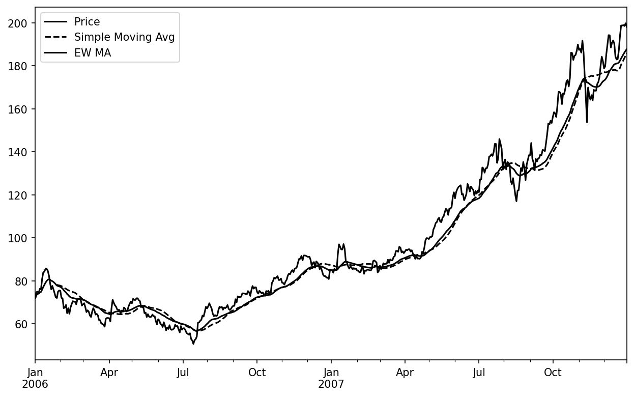
The EMA’s quicker response is not automatically better. Faster adaptation often means more sensitivity to noise. A strategy must test whether a chosen span improves its risk-adjusted, cost-aware behavior rather than assuming that a smoother-looking chart has predictive value.

---

Prevent leakage with a clear decision-time convention

The highest-risk mistake in feature engineering is look-ahead bias: allowing a strategy to use information that did not exist at its claimed decision time.

Suppose you intend to make a decision before the open on session $t$. At that moment, you know data only through the close of session $t-1$. Therefore, every feature must be lagged once.

feature_groups = features.groupby(level="symbol", sort=False)

features["close_prior"] = feature_groups["close_lag_1"].shift(0)
features["sma_20_prior"] = feature_groups["sma_20"].shift(1)
features["vol_20d_prior"] = feature_groups["vol_20d"].shift(1)

features["close_vs_sma_20_prior"] = (
    features["close_prior"] / features["sma_20_prior"] - 1
)

There is a clearer version for close_prior, using the original series:

features["close_prior"] = close.groupby(level="symbol", sort=False).shift(1)

At row $t$, close_prior, sma_20_prior, and vol_20d_prior now contain values known by the prior close. A rule based on those columns is eligible for a pre-open decision on row $t$, subject to the precise execution assumptions that you will formalize later.

By contrast, a negative shift creates a future outcome:

features["forward_ret_1d"] = (
    close.groupby(level="symbol", sort=False).shift(-1) / close - 1
)

This can be useful as an evaluation target: it measures the next session’s close-to-close return. It must never be used as an input feature or trading condition. Its final value for each stock is correctly NaN, because there is no following observed close.

Finally, join the feature table back to your price panel:

research_panel = prices.join(features, how="left", validate="1:1")

research_panel[
    [
        "close",
        "ret_1d",
        "momentum_20d",
        "sma_20",
        "ema_20",
        "vol_20d_annualized",
        "close_vs_sma_20_prior",
    ]
].tail()

This remains a long panel indexed by (symbol, date), now with a reproducible set of derived columns.

---

Implementation checkpoint

Your feature-engineering code should meet these conditions:

• It sorts the (symbol, date) index before any time-series calculation.
• It groups by symbol before computing returns, lags, windows, or EMAs.
• It accepts warm-up NaN values instead of filling them with zero or future values.
• It treats a 20-period window as 20 observations, not 20 calendar days.
• It records whether a feature is available after the current close or before the current session.
• It never uses .shift(-1) output as a trading input.
• It avoids row-wise .apply(axis=1), iterrows(), and manual loops for calculations pandas and NumPy already vectorize.

Move the stable transformations into a reusable module, such as src/swing_research/features.py. A later unit test should use two short, interleaved symbol histories and verify that each symbol’s first return is missing, each return uses its own prior close, and no rolling feature crosses a symbol boundary.

---

Key takeaways

Returns, lags, and rolling statistics are not merely indicator formulas. They are time-alignment operations, and their correctness depends on the grain and ordering of the data.

• Use grouped calculations so every stock’s history is processed independently.
• .pct_change() produces fractional returns; multiply by 100 only for display as percentages.
• Use shift(1) to align prior observations with the current row.
• Calculate rolling averages and volatility with explicit windows and warm-up requirements.
• EMAs weight recent observations more heavily than simple moving averages.
• Shift completed features when the trading decision occurs before the current session’s close.
• Treat negative shifts as future labels for evaluation, never as strategy inputs.

Next, you will handle exchange dates, session boundaries, and Asia/Kolkata timestamps correctly—turning this daily-bar workflow into one that respects the actual Indian market calendar.