Perceptrons: Limitations and the XOR Problem

Recommended resources

The freely available resources this lesson will direct you to.

Introduction

In our last module, we assembled a powerful toolkit for optimization, culminating in the Adam optimizer. We now have sophisticated methods for minimizing a loss function by iteratively updating a model's parameters. However, we have yet to formally define the model itself. We've been working under the assumption of a model with parameters $w$ , but what form does this model take?

We now transition from the how of optimization to the what of architecture. We will start with the foundational building block of all neural networks: the perceptron. Conceived in 1958 by Frank Rosenblatt, the perceptron is a simple computational model inspired by a biological neuron. It serves as the "hydrogen atom" of neural networks, and understanding its function and, more importantly, its limitations is the critical first step toward understanding modern deep learning.

In this lesson, you will learn the mathematical definition of the perceptron and its geometric interpretation as a linear classifier. We will then demonstrate its power by implementing fundamental logic gates. Finally, we will uncover its crucial weakness by proving its inability to solve a classic, non-linearly separable problem: the exclusive OR (XOR) function.

The Perceptron Model

At its core, a perceptron is a simple decision-making unit. It takes a set of numerical inputs, computes a weighted sum, and if that sum exceeds a certain threshold, it "fires" by outputting a 1; otherwise, it outputs a 0.

Let's formalize this. A perceptron with $m$ inputs $(x_{1}, x_{2}, \dots, x_{m})$ has a corresponding set of weights $(w_{1}, w_{2}, \dots, w_{m})$ and a bias term $b$ .

Compute the weighted sum: The first step is to compute the dot product of the input vector $x$ and the weight vector $w$ , and add the bias. We'll call this intermediate value $z$ . $z = (w \cdot x) + b = i = 1 \sum m w_{i} x_{i} + b$
Apply an activation function: The perceptron's output, $o$ , is determined by applying a simple step function (specifically, the Heaviside step function) to $z$ . $o = {10 if z \geq 0 if z < 0$

The bias term, $b$ , can be thought of as adjusting the perceptron's threshold for firing. A higher bias makes it easier to fire (output 1), while a lower (more negative) bias makes it harder. An alternative but equivalent formulation is to treat the bias as a weight $w_{0}$ for a constant input $x_{0} = 1$ . This simplifies the equation to a pure dot product.

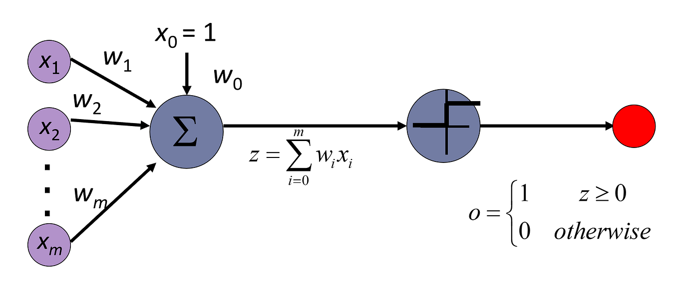
This diagram illustrates the structure of a perceptron. Inputs $x_1$ through $x_m$ are multiplied by their respective weights $w_1$ through $w_m$. The bias is shown as a weight $w_0$ applied to a constant input $x_0=1$. These are summed to produce $z$, which is then passed through a step function to produce the final binary output $o$.

To get a dynamic overview of this process, the following video provides a concise explanation.

Perceptron | Neural Networks

The video "Perceptron | Neural Networks" from the First Principles of Computer Vision channel defines the model and its components.

Please watch the first two minutes, from the beginning. This will walk you through the definition of the inputs, weights, bias, the weighted sum, and the step activation function. Notice that the video uses the condition z > 0 for an output of 1, which is also a common convention. For our purposes, we will stick with z \ge 0.

Geometric Interpretation: The Linear Classifier

The true power of the perceptron lies in its geometric interpretation. The decision rule $\sum w_{i} x_{i} + b = 0$ defines a hyperplane in the input space. For two inputs $(x_{1}, x_{2})$ , this is simply the equation of a line: $w_{1} x_{1} + w_{2} x_{2} + b = 0$ .

This hyperplane acts as a decision boundary.

All input points $x$ on one side of the hyperplane will result in $z \geq 0$ , causing the perceptron to output 1.
All input points on the other side will result in $z < 0$ , causing an output of 0.

Thus, a single perceptron is a linear classifier. It can only learn to separate data points that are linearly separable—that is, two classes of points that can be divided by a single line, plane, or hyperplane.

Perceptron | Neural Networks

The same video provides an excellent visualization of this concept.

Watch the segment from "what a single perceptron is doing". The presenter walks through a concrete example with two inputs, showing how different values of weights and bias define a line that partitions the 2D input space into two regions, one for each output class.

Perceptrons as Logic Gates

To make this concrete, let's see how a perceptron can implement basic Boolean logic gates. This is a classic exercise that reveals both the power and the limitations of the model. We'll consider gates with two binary inputs, $x_{1}, x_{2} \in {0, 1}$ .

Challenge Question:

Consider the AND gate. Its truth table is:

$x_{1}$	$x_{2}$	Output
0	0	0
0	1	0
1	0	0
1	1	1

Can you find a set of weights $w_{1}, w_{2}$ and a bias $b$ for a perceptron that correctly implements this function? Remember the rule: $w_{1} x_{1} + w_{2} x_{2} + b \geq 0$ must be true only for the case where the output should be 1.

Click here for a possible solution and explanation.

A simple solution for the AND gate is $w_{1} = 1$ , $w_{2} = 1$ , and $b = - 1.5$ . Let's check:

(0, 0): $1(0) + 1(0) - 1.5 = -1.5 < 0 \implies 0$ (Correct)
(0, 1): $1(0) + 1(1) - 1.5 = -0.5 < 0 \implies 0$ (Correct)
(1, 0): $1(1) + 1(0) - 1.5 = -0.5 < 0 \implies 0$ (Correct)
(1, 1): $1(1) + 1(1) - 1.5 = 0.5 \ge 0 \implies 1$ (Correct)

Geometrically, the decision boundary is the line $x_1 + x_2 - 1.5 = 0$. This line successfully separates the point (1,1) from the other three points. Note that there are infinitely many other valid solutions.

It turns out that a single perceptron can also implement OR and NAND gates. The following resource demonstrates how.

Neural Networks 2 XOR

The video "Neural Networks 2 XOR" provides worked examples for both AND and OR gates.

Watch the segment from "build a Perceptron". It walks through the calculations for specific weight and bias values for AND and OR, confirming that they produce the correct outputs for all input combinations.

The ability to implement a NAND gate is particularly significant. As you know from your computer science background, the NAND gate is functionally complete, meaning any Boolean function can be constructed by networking NAND gates together. This implies that a network of perceptrons is capable of universal computation, a profound result that laid the groundwork for modern neural networks.

The Achilles' Heel: Non-Linear Separability

We've established that a perceptron is a linear classifier. This brings us to its fundamental limitation. What happens if a problem is not linearly separable?

The canonical example is the XOR (exclusive OR) gate.

$x_{1}$	$x_{2}$	Output
0	0	0
0	1	1
1	0	1
1	1	0

Let's visualize the input points, colored by their desired output class.

This figure shows the 2D input space for NAND, OR, and XOR gates. For NAND and OR, the 'Class 1' points can be separated from the 'Class 0' points by a single straight line. For XOR, the 'Class 1' points (0,1) and (1,0) cannot be separated from the 'Class 0' points (0,0) and (1,1) by a single line.

As the image clearly shows, there is no single line you can draw to separate the points that should output 1 from the points that should output 0. The XOR function is not linearly separable. This visual intuition is powerful, but for a "first principles" understanding, we need a formal proof.

One elegant proof uses basic coordinate geometry to show a contradiction.

Is there a proof to explain why XOR cannot be linearly separable?

This StackExchange answer provides a concise proof by contradiction.

Read the second answer on the page, which starts with the coordinate geometry proof. The logic is as follows: Assume a separating line ax+by+c=0 exists. Use the property that points on the same side of the line, when plugged into the line's equation, yield results with the same sign. Points on opposite sides yield results with opposite signs. Write down the inequalities that must hold for the four XOR data points based on this property. Show that these inequalities lead to a mathematical contradiction, proving the initial assumption (the existence of the line) must be false.

Another, more algebraic proof is also common.

[PDF] Threshold Logic Units - Computational Intelligence Book

The textbook chapter "Threshold Logic Units" by Christian Borgelt provides a similar proof for the XNOR (biimplication) problem, which is logically equivalent to XOR with flipped outputs.

Focus on the section titled "The biimplication problem". The proof establishes four inequalities based on the four input cases and shows they cannot all be true simultaneously. You can adapt this proof directly to the XOR case by flipping the signs of the inequalities.

The failure of the perceptron to solve the XOR problem was a significant event in the history of AI. It highlighted a major limitation and contributed to a period of reduced funding and interest in neural networks, often called the first "AI winter." It became clear that to tackle more complex problems, a more powerful model was needed.

Conclusion

In this lesson, we have dissected the original perceptron model. We've seen its elegant simplicity and understood its operation both algebraically and geometrically.

Key Takeaways:

Perceptron Model: A perceptron computes a weighted sum of its inputs, adds a bias, and passes the result through a step function to produce a binary output.
Linear Classifier: Geometrically, a perceptron functions as a linear classifier. The equation $w^{T} x + b = 0$ defines a decision boundary (a hyperplane) that divides the input space into two regions.
Capabilities: A single perceptron can solve any linearly separable problem, including implementing logic gates like AND, OR, and NAND. Because NAND is functionally complete, a network of perceptrons can, in principle, perform any logical computation.
The XOR Limitation: The perceptron's primary weakness is its inability to solve non-linearly separable problems. The classic example is the XOR function, for which no single linear decision boundary can correctly classify all four input points.

The limitation of a single perceptron is not the end of the story, but rather the motivation for what comes next. If one line is not enough, perhaps we can combine multiple lines? Or, more powerfully, what if we could learn to map the points into a new space where they are linearly separable?

Preview of the Next Lesson:

The step function used by the perceptron is harsh and non-differentiable, making it unsuitable for the gradient-based optimization methods we have studied. To build networks that can learn complex, non-linear functions, we need smoother "activation functions." In the next lesson, we will introduce modern activation functions like Sigmoid, Tanh, and the ubiquitous ReLU, and compute their derivatives—a crucial step towards building differentiable, multi-layer neural networks.