Activation Functions and Their Derivatives

Introduction

In our previous lesson, we explored the perceptron and established its fundamental limitation: its reliance on a non-differentiable step function. This "all-or-nothing" activation makes it incompatible with the gradient-based optimization methods we have studied, as the zero-gradient landscape offers no guidance for learning. This isn't merely an inconvenience; it's a hard barrier that prevented early models from learning complex, non-linear patterns.

To move forward and build networks capable of solving problems like XOR and beyond, we must replace the rigid step function with a smoother alternative. This lesson introduces the modern activation functions that form the bedrock of deep learning: Sigmoid, hyperbolic tangent (Tanh), and the now-ubiquitous Rectified Linear Unit (ReLU). We will define each function mathematically, analyze its properties, and, most critically, compute its derivative. Understanding these derivatives is the essential next step toward deriving the backpropagation algorithm, the engine that powers neural network training.

From Step Function to Smooth Activation

The core issue with the Heaviside step function used in the perceptron is that its derivative is zero everywhere except at the origin, where it is undefined. A gradient of zero provides no information to an optimizer like SGD; it cannot determine whether to increase or decrease a weight to reduce the loss. We need functions that are sensitive to changes in their input, providing a non-zero, informative gradient.

The Sigmoid Function

The first natural replacement for the step function is the sigmoid or logistic function. It provides a smooth, 'S'-shaped curve that squashes any real-valued input $z$ into the range $(0,1)$.

Its mathematical form is:

This output can be conveniently interpreted as a probability, making it a historical favorite for the output layer of binary classification models.

Before we derive its derivative, let's consider the mechanics. Given the function's form as a fraction with an exponential term in the denominator, which calculus rules would you need to apply to find $\frac{d}{dz}\sigma (z)$?

Let's walk through the derivation using the chain rule, which is often more intuitive in the context of nested functions in neural networks.

As you saw in the video, the derivative of the sigmoid function simplifies beautifully:

This is a powerful result. From a computational standpoint, if you have already calculated the output of the sigmoid function, $\sigma (z)$, during the forward pass of a neural network, you can reuse that value to compute its derivative almost for free. There is no need for another expensive exp calculation. If we let $a=\sigma (z)$, then the derivative is simply $a(1-a)$.

The Vanishing Gradient Problem

Despite its elegance, the sigmoid function has a significant drawback. Let's examine its derivative visually.

When the input $z$ is very large or very small, the sigmoid function saturates, and its gradient becomes extremely close to zero. During backpropagation (which we will cover in detail later), these tiny gradients get multiplied through many layers. This can cause the overall gradient signal for the weights in the early layers of the network to "vanish," effectively stopping them from learning. This is the infamous vanishing gradient problem.

The Hyperbolic Tangent (Tanh)

A close relative of the sigmoid is the hyperbolic tangent, or tanh, function. It also has an 'S' shape but squashes inputs to the range $(-1,1)$.

Its mathematical form is:

Being zero-centered (i.e., its range is symmetric around zero) is a key advantage over sigmoid. This property tends to help with optimization by keeping the activations from different layers on a more consistent scale.

The derivation of its derivative follows a similar pattern to the sigmoid's, resulting in another computationally efficient form.

The derivative of the tanh function is:

Like the sigmoid, if we have already computed $a=\tanh (z)$, the derivative is simply $1-a^2$. The gradient of tanh is steeper than that of sigmoid around the origin (1 vs. 0.25), which can lead to faster initial learning. However, it also suffers from the vanishing gradient problem as its output saturates towards -1 or 1.

The Rectified Linear Unit (ReLU)

The vanishing gradient problem of sigmoid and tanh led researchers to seek alternatives. The solution turned out to be remarkably simple: the Rectified Linear Unit, or ReLU. It has become the default activation function for hidden layers in most neural networks today due to its simplicity and effectiveness.

The function is defined as:

In words, the output is simply the input if the input is positive, and zero otherwise.

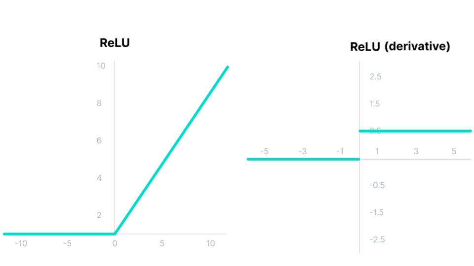
This piecewise nature raises a critical question for a "first principles" approach. The function is clearly not "smooth" at $z=0$. Is it differentiable there?

As the article explains, the derivative of ReLU is undefined at $z=0$. However, in practice, the probability of hitting $z=0$ exactly with floating-point arithmetic is negligible. We can simply assign a value for the derivative at that point, usually 0 or 1. The optimization process is robust to this technicality.

So, for practical purposes, the derivative, $g^{\prime }(z)$, is:

Advantages of ReLU:

• Computational Efficiency: It involves a simple max operation, which is much faster than the exp calls in sigmoid and tanh. This is a significant consideration for performance in low-level implementations.
• No Vanishing Gradient (for positive inputs): For positive inputs, the gradient is a constant 1. This allows the gradient signal to propagate back through many layers without shrinking, greatly alleviating the vanishing gradient problem.

Disadvantage of ReLU:

• The "Dying ReLU" Problem: If a neuron's input is consistently negative, its output will be zero, and therefore its gradient will also be zero. This neuron will stop learning entirely, as its weights will no longer be updated.

To address this, variants like Leaky ReLU were introduced. It has a small, non-zero slope for negative inputs: $f(z)=\max (\alpha z,z)$, where $\alpha$ is a small constant like 0.01. This ensures the neuron never completely "dies."

Conclusion

In this lesson, we have armed ourselves with the essential non-linear tools needed to build modern neural networks. We have moved from the perceptron's non-differentiable step function to a set of smoother, more practical alternatives.

Key Takeaways:

• Activation's Role: Activation functions introduce the non-linearity that allows neural networks to learn complex patterns beyond what a simple linear model can capture.
• Sigmoid & Tanh: These are 'S'-shaped functions that squash inputs into a finite range. While historically important, they suffer from the vanishing gradient problem where their derivatives approach zero in saturated regions, impeding learning.
• ReLU: The Rectified Linear Unit ($\max (0,z)$) is the modern default. It is computationally cheap and avoids vanishing gradients for positive inputs, but can suffer from the "dying ReLU" problem for negative inputs.
• Derivatives as a Function of Output: For both sigmoid ($a(1-a)$) and tanh ($1-a^2$), the derivative can be calculated efficiently using the function's output ($a$). The derivative of ReLU is a simple piecewise constant. These efficient calculations are crucial for the implementation of backpropagation.

We have now defined the two primary components of a neural network layer: an affine transformation ($\mathbf{Wx}+\mathbf{b}$) and a non-linear activation function ($g(z)$). We are finally ready to stack these layers together.

Preview of the Next Lesson:

In the next lesson, we will formally construct a multi-layer feedforward neural network by composing these components. We will define the full forward pass, where an input signal propagates through the network to produce a final prediction. This will set the stage for understanding how we compare that prediction to a target and, ultimately, how we compute the gradients to train the model.