Backpropagation Through an Affine–ReLU Layer

Welcome back. In the previous lesson, a Jacobian described how a small input displacement changes a transformation’s output. Now we will use that same derivative information in reverse: given a scalar loss, how does a change in a layer’s input, weights, or bias affect it?

You will derive the backward pass for an affine layer followed by a ReLU, then check the result against PyTorch autograd. This is a foundation for training the networks you will later apply to 3D points and other geometric data. Allow about 40 minutes, including the video, reading, and code check.

Why gradients travel backward

Consider a layer with input $\mathbf{x}$, weights $W$, and bias $\mathbf{b}$:

Suppose later computations produce a scalar loss $J$. We could try to write $J$ directly as one enormous expression in every parameter, but that becomes unwieldy as layers are added. Reverse-mode differentiation instead starts with the effect of $\mathbf{a}$ on $J$, then uses each operation’s local derivative to work back toward its inputs.

There are two kinds of quantities to keep distinct. The incoming gradient tells us how the final loss responds to the output of the operation we are examining. A local derivative tells us how that operation’s output responds to one of its inputs. Their chain-rule combination gives the gradient needed by the preceding operation.

Set the shapes and convention

Let $\mathbf{x}\in {\mathbb{R}}^n$, $\mathbf{z},\mathbf{a},\mathbf{b}\in {\mathbb{R}}^m$, and $W\in {\mathbb{R}}^{m\times n}$. We will write vectors, including gradients, as columns. Assume that the rest of the network has supplied

Our task is to obtain ${\nabla }_{\mathbf{x}}J$, ${\nabla }_{W}J$, and ${\nabla }_{\mathbf{b}}J$. The backward pass must first cross ReLU and then the affine operation, because ReLU was applied last in the forward calculation.

The following reading develops the same two local backward rules. It uses row gradients in much of its linear-layer derivation, so pay particular attention to orientation: a transposed formula may express the same result under our column-gradient convention.

Derive the backward pass

ReLU acts independently on each component:

For $z_i>0$, its local derivative is one; for $z_i<0$, it is zero. At $z_i=0$, ReLU is not differentiable. We will choose a backward value of zero there, matching PyTorch. Define the componentwise mask $r_i=1_{\{z_i>0\}}$. The gradient arriving at the input of ReLU is therefore

where $\odot$ means componentwise multiplication. A negative pre-activation blocks that component’s incoming gradient, even if the incoming gradient itself is large.

Now examine the affine operation component by component:

A weight $W_{ij}$ affects $z_i$ at a rate of $x_j$, so the chain rule gives

Collecting these entries produces an outer product. The bias $b_i$ changes $z_i$ at a rate of one. An input $x_j$, meanwhile, contributes to every $z_i$, so its gradient sums contributions across output components:

The shapes check the calculation: $\mathbf{\delta }{\mathbf{x}}^{\mathsf{T}}$ is $m\times n$, $W^{\mathsf{T}}\mathbf{\delta }$ has $n$ entries, and the bias gradient has $m$ entries.

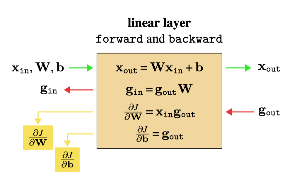
This also connects directly to the previous lesson. Where ReLU is differentiable, its Jacobian is the diagonal matrix $\mathrm{diag}(\mathbf{r})$. The Jacobian of the combined map from $\mathbf{x}$ to $\mathbf{a}$ is $\mathrm{diag}(\mathbf{r})W$. Reverse-mode differentiation applies its transpose to $\mathbf{u}$, yielding $W^{\mathsf{T}}\mathbf{\delta }$. In practice, we do not build the diagonal matrix: multiplying by its entries as a mask is simpler.

For a quick numerical check, take $\mathbf{x}=(1,-1{)}^{\mathsf{T}}$,

The forward pass gives $\mathbf{z}=(1,-1.5{)}^{\mathsf{T}}$, so $\mathbf{\delta }=(3,0{)}^{\mathsf{T}}$. Thus

The second ReLU output contributes no gradient to this layer’s weights or bias for this input. The first output still sends a gradient to both input coordinates because it depends on both.

Check a batch against autograd

PyTorch typically stores one input per row of a batch matrix $X\in {\mathbb{R}}^{B\times n}$. If $W$ retains shape $m\times n$, the forward affine calculation is X @ W.T + b. The bias is shared across rows, so its gradient is the sum of their contributions. Writing $G\in {\mathbb{R}}^{B\times m}$ for the ReLU-masked incoming gradients, the batched results are

This is the same single-input rule applied to each row, with shared-parameter gradients added together. If the loss were a mean over the batch rather than a sum, its incoming gradients—and consequently these parameter gradients—would include the appropriate averaging factor.

Run the following as one block. The simple scalar $J$ supplies known incoming gradients; it is a gradient check, not a training objective.

import torch

dtype = torch.float64
X = torch.tensor(
    [[1.0, -1.0, 2.0],
     [-1.0, 0.0, 0.0]],
    dtype=dtype, requires_grad=True,
)
W = torch.tensor(
    [[1.0, -1.0, 0.5],
     [-2.0, 0.0, 1.0]],
    dtype=dtype, requires_grad=True,
)
b = torch.tensor([0.1, -0.2], dtype=dtype, requires_grad=True)

# An explicitly chosen incoming gradient for each ReLU output.
U = torch.tensor(
    [[2.0, -3.0],
     [4.0, 5.0]],
    dtype=dtype,
)

Z = X @ W.T + b
A = torch.relu(Z)
J = (A * U).sum()
J.backward()

# Derive the same gradients without using autograd on these expressions.
G = U * (Z.detach() > 0).to(dtype)
manual_dX = G @ W.detach()
manual_dW = G.T @ X.detach()
manual_db = G.sum(dim=0)

torch.testing.assert_close(X.grad, manual_dX)
torch.testing.assert_close(W.grad, manual_dW)
torch.testing.assert_close(b.grad, manual_db)

print("pre-activations:\n", Z.detach())
print("masked gradients:\n", G)
print("weight gradient:\n", manual_dW)
print("bias gradient:", manual_db)
print("input gradient:\n", manual_dX)

The two batch rows activate different ReLU components. You should see a weight gradient of [[2, -2, 4], [-5, 0, 0]] and a bias gradient of [2, 5]. Notice that the code needs saved forward values to determine the ReLU mask and to form the weight gradient. None of the pre-activations here equals zero, so the gradient check does not depend on the chosen convention at that kink.

Takeaways

Reverse-mode differentiation combines an incoming loss gradient with local derivatives, working from ReLU back through the affine layer. ReLU masks the gradient componentwise; the affine layer sends $W^{\mathsf{T}}\mathbf{\delta }$ to its input and produces an outer-product weight gradient and a bias gradient. For batches, shared-parameter contributions are summed.

You can now explain the gradients that autograd computes rather than treating .backward() as a black box. Next, you will use parameter gradients to implement gradient-descent and Adam updates, including how to recognize an unstable learning rate.