Gradient Descent, Adam, and Learning Rate Stability

Welcome back. In the previous lesson, you computed gradients for an affine layer followed by ReLU and checked them against autograd. A gradient tells you how a loss changes locally; an optimizer decides how to use that information to change the parameters.

This lesson takes you from gradients to updates. You will implement gradient descent and Adam in PyTorch, then use a small loss landscape to identify when a learning rate is too large. The same update machinery will train your first multilayer perceptron in the next lesson and, later, models for 3D data. Allow about 40 minutes, including the videos and code.

---

From a gradient to a parameter update

Let $\mathbf{\theta }$ collect a model’s trainable parameters, and let $J(\mathbf{\theta })$ be its loss. At each step, gradient descent evaluates the gradient at the current parameters and moves in the opposite direction:

$${\mathbf{\theta }}_t={\mathbf{\theta }}_{t-1}-\eta \nabla J({\mathbf{\theta }}_{t-1}).$$

The positive number $\eta$ is the learning rate. It scales the update, not the gradient calculation. A small learning rate can make progress needlessly slow; a large one can jump across a minimum and increase the loss.

PyTorch’s autograd supplies the gradient, but a manual update still needs care: change the parameter without recording the update as part of the computation graph, and clear its stored gradient before the next backward pass. The following video shows those mechanics in a one-parameter example.

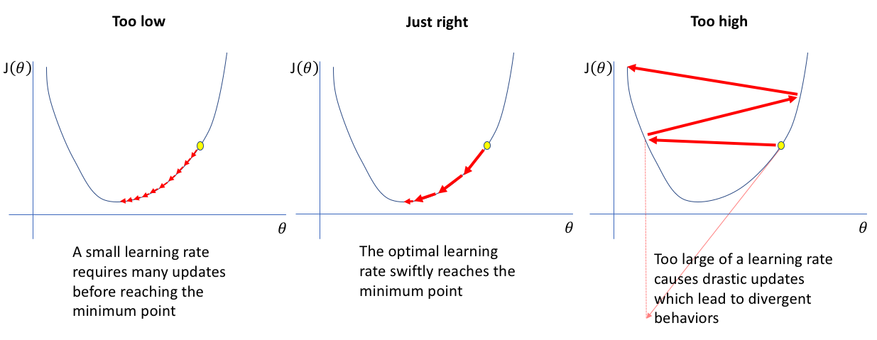
The picture is useful, but “too high” is not simply “a step crossed the minimum.” A step can cross it and still end up closer. To see the distinction, consider the one-dimensional quadratic

$$J(\theta )=\frac{a}{2}(\theta -{\theta }^{\star }{)}^2,a>0.$$

Its gradient is $a(\theta -{\theta }^{\star })$. If $e_t={\theta }_t-{\theta }^{\star }$ denotes the error after an update, gradient descent gives

$$e_t=(1-\eta a)e_{t-1}.$$

Thus the error shrinks when $|1-\eta a|<1$, or $0<\eta <2/a$. It alternates sides of the minimum when $1/a<\eta <2/a$, yet still converges. Above $2/a$, those alternating errors grow. This is an exact result for this quadratic, not a universal learning-rate formula for neural networks. It does show why the scale of the loss’s curvature matters.

---

Adam: direction and scale from recent gradients

Ordinary gradient descent uses the current gradient alone. Adam keeps two running, elementwise summaries of past gradients: one for their signed direction and one for their squared magnitude. Watch the conceptual explanation before implementing it.

Using $t=1$ for the first update, let ${\mathbf{g}}_t=\nabla J({\mathbf{\theta }}_{t-1})$. Adam starts with ${\mathbf{m}}_0={\mathbf{v}}_0=0$ and computes

$$\begin{array}{rl}{\mathbf{m}}_t& ={\beta }_1{\mathbf{m}}_{t-1}+(1-{\beta }_1){\mathbf{g}}_t,\\ {\mathbf{v}}_t& ={\beta }_2{\mathbf{v}}_{t-1}+(1-{\beta }_2){\mathbf{g}}_t^2,\\ {\hat{\mathbf{m}}}_t& =\frac{{\mathbf{m}}_t}{1-{\beta }_1^t},{\hat{\mathbf{v}}}_t=\frac{{\mathbf{v}}_t}{1-{\beta }_2^t},\\ {\mathbf{\theta }}_t& ={\mathbf{\theta }}_{t-1}-\eta \frac{{\hat{\mathbf{m}}}_t}{\sqrt{{\hat{\mathbf{v}}}_t}+ϵ}.\end{array}$$

Squares, roots, and division here are elementwise. Common starting choices are ${\beta }_1=0.9$, ${\beta }_2=0.999$, and $ϵ=10^{-8}$. The first running average follows the direction of recent gradients; the second helps scale updates separately for each parameter component. The small $ϵ$ prevents division by zero.

Why divide by $1-{\beta }_1^t$ and $1-{\beta }_2^t$? Both averages started at zero, so their early values are pulled toward zero. These bias corrections compensate for that initialization. On the first step, for example, they yield ${\hat{\mathbf{m}}}_1={\mathbf{g}}_1$ and ${\hat{\mathbf{v}}}_1={\mathbf{g}}_1^2$.

Adam does not remove the need to choose a learning rate. Nor should you expect either optimizer to lower the loss on every step of a noisy training run.

---

Implement both updates

We will optimize a two-component parameter rather than a neural network so that the behavior is easy to inspect. The minimum of this loss is at $(1,2)$:

$$J(\mathbf{\theta })=\frac{1}{2}\left[({\theta }_1-1{)}^2+10({\theta }_2-2{)}^2\right].$$

The second direction is ten times more curved than the first. For gradient descent on this particular loss, the earlier quadratic calculation says both components shrink only if $0<\eta <0.2$. The code uses autograd for gradients but implements both parameter updates explicitly.

import torch

def objective(theta):
    target = torch.tensor([1.0, 2.0], dtype=theta.dtype)
    curvature = torch.tensor([1.0, 10.0], dtype=theta.dtype)
    return 0.5 * (curvature * (theta - target).square()).sum()

def gd_step(params, lr):
    with torch.no_grad():
        for p in params:
            if p.grad is None:
                raise ValueError("Compute every parameter gradient before updating.")
            p.add_(p.grad, alpha=-lr)

def init_adam(params):
    return {
        "step": 0,
        "m": [torch.zeros_like(p) for p in params],
        "v": [torch.zeros_like(p) for p in params],
    }

def adam_step(params, state, lr, beta1=0.9, beta2=0.999, eps=1e-8):
    state["step"] += 1
    t = state["step"]

    with torch.no_grad():
        for p, m, v in zip(params, state["m"], state["v"]):
            if p.grad is None:
                raise ValueError("Compute every parameter gradient before updating.")
            g = p.grad
            m.mul_(beta1).add_(g, alpha=1 - beta1)
            v.mul_(beta2).addcmul_(g, g, value=1 - beta2)

            m_hat = m / (1 - beta1**t)
            v_hat = v / (1 - beta2**t)
            p.add_(-lr * m_hat / (v_hat.sqrt() + eps))

def run(method, lr, steps=25):
    theta = torch.tensor([3.0, -3.0], dtype=torch.float64,
                         requires_grad=True)
    params = [theta]
    state = init_adam(params) if method == "adam" else None
    losses = []

    for _ in range(steps):
        # backward() accumulates gradients; start this step with none.
        for p in params:
            p.grad = None

        loss = objective(theta)
        losses.append(loss.item())
        loss.backward()

        if method == "gd":
            gd_step(params, lr)
        else:
            adam_step(params, state, lr)

    with torch.no_grad():
        losses.append(objective(theta).item())
        final_theta = theta.clone()
    return final_theta, losses

# Check the first updates against values calculated directly.
gd_theta, _ = run("gd", 0.05, steps=1)
adam_theta, _ = run("adam", 0.1, steps=1)
torch.testing.assert_close(
    gd_theta, torch.tensor([2.9, -0.5], dtype=torch.float64)
)
torch.testing.assert_close(
    adam_theta, torch.tensor([2.9, -2.9], dtype=torch.float64),
    rtol=1e-7, atol=1e-7,
)

for method, lr in [
    ("gd", 0.005), ("gd", 0.05), ("gd", 0.25), ("adam", 0.25)
]:
    theta, losses = run(method, lr)
    print(f"{method:4s} lr={lr:.3f}  "
          f"losses at steps 0, 1, 10, 25: "
          f"{[round(losses[i], 3) for i in (0, 1, 10, 25)]}  "
          f"final theta={theta.tolist()}")

The first-update checks catch several common mistakes. Initially, the gradient is $(2,-50)$. Gradient descent with $\eta =0.05$ therefore changes the parameters from $(3,-3)$ to $(2.9,-0.5)$. Adam’s bias-corrected first step with $\eta =0.1$ changes each component by approximately $0.1$ in the direction opposite its gradient, giving $(2.9,-2.9)$.

In the longer runs, expect gradient descent at $0.005$ to make slow progress, $0.05$ to reduce the loss, and $0.25$ to grow unstable. Adam at $0.25$ may behave quite differently on this example because it rescales components—but that is not a promise that $0.25$ is safe for Adam on another loss. Notice also that each new run creates fresh parameters and fresh Adam state. Carrying moment estimates over to an unrelated run would change the experiment.

---

Diagnose an unstable learning rate

On the toy loss, the diagnosis is unusually clear: the component with curvature $10$ multiplies its error by $1-10\eta$ each gradient-descent step. At $\eta =0.25$, that factor is $-1.5$: the component crosses the minimum and moves farther away each time. Its loss contribution consequently grows.

Real training curves are less tidy. Minibatches produce varying gradients, and a single upward loss step is not proof of instability. Look instead for sustained or repeated sharp rises, widening oscillations, or non-finite losses or parameters. Compare runs from the same initialization while changing the learning rate; log the loss frequently enough to see early behavior. If a large gradient spike accompanies a loss spike, the gradient norm can help locate the problem.

For a short, practical discussion of what to monitor, read the following excerpt.

A useful first response to suspected learning-rate instability is to lower the learning rate and rerun the same setup. If that produces a substantially steadier loss curve, the comparison supports the diagnosis. Gradient clipping or a learning-rate warmup can address particular patterns, but neither substitutes for checking the update scale; clipping nearly every update can simply disguise an overly large rate.

---

Takeaways

Gradient descent subtracts a learning-rate-scaled current gradient. Adam also maintains running averages of gradients and squared gradients, corrects their initial bias, and scales updates componentwise. In PyTorch, manual updates belong inside torch.no_grad(), and gradients must be cleared between backward passes.

The learning rate determines whether useful local gradient information becomes steady progress, slow progress, or unstable jumps. You now have both update rules and a way to inspect their behavior. Next, you will put the loss, backpropagation, and an optimizer together to train a small multilayer perceptron.