Recommended resources
The freely available resources this lesson will direct you to.
- Understanding NVIDIA GPU Hardware as a CUDA C Programmer | Episode 2: GPU Compute Architecturewww.youtube.com
- GPU Warps Explained: How SIMT Really Works Under the Hood (Visual Deep Dive) | M2L3www.youtube.com
- CUDA Best Practices Guide - NVIDIA Documentation Hubdocs.nvidia.com
- Kernel Profiling Guidedocs.nvidia.com
Hello! Last time, you followed a CUDA kernel from its grid through blocks and warps to instruction issue on an SM. One distinction matters especially now: a warp can be resident without issuing an instruction in a given cycle. This lesson explains what the SM does when a resident warp must wait—and why keeping other warps available can preserve throughput without making the delayed instruction itself faster.
The latency-hiding idea
Consider a warp that issues a global-memory load and then needs the loaded value for an addition. The addition cannot use a value that has not arrived. But the load does not have to occupy an arithmetic pipeline throughout its wait. If another warp has an instruction ready, a warp scheduler can issue that instruction instead.
Watch this short illustration of the mechanism:
Understanding NVIDIA GPU Hardware as a CUDA C Programmer | Episode 2: GPU Compute Architecture
Watch “Understanding NVIDIA GPU Hardware as a CUDA C Programmer,” by Tushar Gautam, for its visual explanation of keeping other work ready while memory requests are outstanding.
Watch warp switching. Focus on the resident execution state and the choice to run other work during a delay. The narration sometimes says “threads” or “cores”; for our performance model, track the warp being selected to issue rather than imagining an operating-system thread switch or a guarantee about a particular core.
A useful distinction is between latency and throughput. Latency is how long a particular result takes to become usable. Throughput is how much work the SM completes over time. Scheduling another warp generally does not shorten the first warp’s memory request. It can, however, fill cycles that would otherwise have no useful instruction to issue.
That switch is relatively cheap because an active warp’s execution state remains resident. The scheduler does not need to save one warp’s registers to memory and restore another’s merely to alternate between their instructions. There are still limits on how many warps can be resident; for now, the key point is that resident work provides a pool from which schedulers can choose.
Resident, eligible, and issuing are different states
The picture below shows an SM organized into scheduler-associated processing areas, with register files, execution pipelines, and paths toward memory. Treat its component counts and layout as an architecture-specific illustration, not a specification for every GPU.
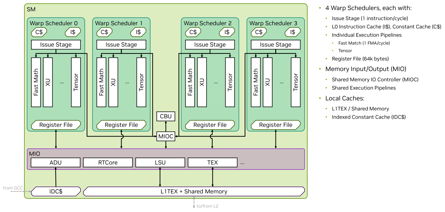
The Kernel Profiling Guide gives more precise vocabulary for this picture:
Read the “Streaming Multiprocessor” discussion in the Kernel Profiling Guide to distinguish warps that occupy hardware resources from warps that can actually issue.
In “Streaming Multiprocessor” (printed p. 19), begin where the discussion says “Each SM is partitioned into four processing blocks.” Read the scheduler discussion through the list ending with “a synchronization barrier.” Pay particular attention to the definitions of active or resident and eligible, and to the stated reasons a warp may be stalled. The partition and warp-pool counts describe the architectures discussed in this guide; retain the distinction between states rather than memorizing those counts.
A resident (or active) warp has been allocated execution resources on the SM. An eligible warp is resident and ready to issue an instruction: its instruction is available, its required inputs are ready, and the relevant execution resource can accept it. An issuing warp is one the scheduler actually selects. Consequently, several warps can be resident, fewer can be eligible, and fewer still may issue in a particular cycle.
This is why “the SM has many active warps” is not the same as “the SM has useful work ready every cycle.” A warp might be waiting for a loaded operand, the result of an earlier arithmetic instruction, or sibling warps at a barrier. Conversely, if multiple warps are eligible, the scheduler can choose among them; a ready warp that is not selected has not suffered a data dependency merely because it did not issue that cycle.
Scheduling happens among the warps available to the relevant scheduler or sub-partition, not by freely moving a warp to any execution unit anywhere on the GPU. That qualification matters when reasoning from an SM-wide warp count to a particular pipeline’s ability to stay busy.
Hiding an instruction dependency
Latency hiding applies to arithmetic as well as memory. Suppose, in a deliberately simplified example, a warp issues an arithmetic instruction in cycle 0 and its next instruction depends on that result. Assume the result becomes usable in cycle 4, and that one scheduler has one issue opportunity per cycle. If warps B, C, and D each have a ready instruction, the issue opportunities can look like this:
| Cycle | Instruction the scheduler can issue |
|---|---|
| 0 | Warp A: produce a result |
| 1 | Warp B: ready instruction |
| 2 | Warp C: ready instruction |
| 3 | Warp D: ready instruction |
| 4 | Warp A: use its result |
The dependency took four cycles for A, but it created no empty issue opportunity in this example. This is a model of interleaving, not a promise about an actual device’s issue width, arithmetic latency, or scheduler policy.
The CUDA Best Practices Guide connects this example to register dependencies and to the number of warps available:
CUDA Best Practices Guide - NVIDIA Documentation Hub
Read Sections 11.1–11.3 of the CUDA Best Practices Guide for the relationship between active warps, dependency latency, and execution configuration.
In Section 11.1, “Occupancy,” start with “Thread instructions are executed sequentially in CUDA.” Read the occupancy explanation to its closing sentence about memory latency. Then, in Section 11.2, “Hiding Register Dependencies,” read the dependency example. Its arithmetic latency is explicitly tied to the stated compute capability, not universal. Finally, in Section 11.3, “Thread and Block Heuristics,” start at “Latency hiding and occupancy depend on the number of active warps per multiprocessor” and read the configuration discussion. Focus on why additional active warps can help yet do not guarantee additional performance.
There is a second way to make progress during a dependency: independent instructions within the same warp. If a warp can issue another instruction that does not need the pending result, it may have useful work before returning to the dependent instruction. The compiler’s instruction ordering and the dependencies in the code affect whether that opportunity exists. Thus, the simplified table assumes A has no such instruction ready; real scheduling can exploit both other warps and independent work within a warp.
Why memory latency needs a larger pool of work
Return to the add kernel from the previous lesson. A warp needs values from a and b before it can calculate its output. Once its loads are issued, the memory system can service them while the scheduler issues instructions from other eligible warps—perhaps address calculations or loads for other parts of the grid.
Memory waits can be much longer and more variable than the short arithmetic dependency in the table. Imagine a scaled-down model in which four resident warps each issue one load, each immediately needs its loaded value, and each value takes twelve cycles to arrive. With one load issued per cycle, the four warps can supply issues in cycles 0–3. They cannot fill every opportunity until the first result is ready in cycle 12. Adding ready, independent work could fill some of that gap; merely having four resident warps could not.
The example illustrates a general condition: latency is well hidden only when schedulers have enough eligible work over the duration of the wait. More resident warps increase the potential supply, but do not ensure it. Warps may all reach a dependency or a barrier at roughly the same time, or an execution pipeline may be unable to accept their next instructions.
There is also an important limit to the benefit. If requests arrive faster than the memory system can serve them, issuing more requests can increase queueing rather than improve completed-work throughput. Warp scheduling can overlap waits; it cannot manufacture memory bandwidth. Similarly, once a scheduler already has enough eligible instructions to keep the needed pipelines busy, additional resident warps may add no benefit.
Reading a performance observation without overclaiming
For profiling, keep three questions separate:
- How many warps are resident? This describes the pool of potential work, subject to the kernel’s resources and the device’s limits.
- How many are eligible? This describes whether that pool currently has instructions ready for scheduling.
- How many instructions issue? This describes what the scheduler actually manages to send onward.
Suppose a scheduler repeatedly has resident warps but few eligible ones. That is consistent with latency or synchronization leaving too little ready work; the resident count alone has not solved the problem. If it frequently has multiple eligible warps while continuing to issue, some warps may wait to be selected without leaving an issue slot idle. Neither observation, on its own, identifies the best code change. Pipeline demand, instruction dependencies, memory behavior, and measurement context still matter.
Occupancy expresses active warps as a fraction of the architectural maximum; it is a capacity measure, not a direct measure of eligibility or useful issue. A change that raises occupancy can improve latency tolerance when ready work was scarce. But forcing occupancy higher can also reduce resources available to each thread, and performance need not improve once there is already enough work to cover the relevant waits. In the next lesson, you will calculate what limits occupancy; here, its role is to explain why the scheduler may—or may not—have alternatives when a warp stalls.
Takeaways
Warp scheduling hides latency by issuing ready instructions from other resident warps while one warp waits. It can cover short instruction dependencies and longer memory waits without reducing the latency of the delayed result itself. The mechanism works only when there is eligible work and an appropriate issue opportunity; resident-warps, eligible-warps, and issuing-warps counts answer different questions.
Next, we will calculate how thread count, registers, shared memory, and architectural limits determine the size of that resident warp pool.