Critical Exponents: Characterizing Critical Points

Hello! Welcome to the first lesson of our new module on Scaling and Universality.

In our previous module, we concluded by establishing the Landau-Ginzburg functional as a universal effective field theory. Its power lies in capturing the physics of a phase transition based only on general principles like symmetry and dimensionality, independent of microscopic details. However, we also saw that a simple mean-field analysis of this functional fails for dimensions $d\le 4$, predicting incorrect critical behavior.

This brings us to a crucial question: how do we precisely describe and quantify the correct universal behavior observed in experiments and simulations near a critical point? Today's lesson answers this by formally defining the standard set of critical exponents. These exponents are the quantitative language of critical phenomena—a set of universal numbers that act as the unique "fingerprint" for a given universality class.

The Puzzle of Universal Numbers

As we've discussed, systems as different as a magnet near its Curie point and a fluid near its critical point exhibit strikingly similar behavior. This universality isn't just qualitative; it's quantitative. Experiments measure the same singular behavior, characterized by a set of exponents.

To begin, let's watch a segment of a lecture by Prof. Mehran Kardar that introduces this concept and presents some real experimental data.

The key takeaway is that a small set of exponents universally characterizes the physics at criticality, and our simplest theoretical approach—mean-field theory—fails to predict their values correctly. This motivates us to define these exponents rigorously, as they are the fundamental quantities any successful theory of critical phenomena must be able to explain.

Formal Definitions of Critical Exponents

To provide a precise framework, we define our variables relative to the critical point $(T_c,h_c)$. We use the reduced temperature, $t$, and the ordering field, $h$:

$t=\frac{T-T_c}{T_c}$
$h=H-H_c$

For a simple magnet, $H$ is the external magnetic field, and the critical field $H_c$ is typically zero. The order parameter is the magnetization, $m$.

The singular behavior of various thermodynamic and correlation functions as $t\to 0$ and $h\to 0$ is described by power laws, whose exponents are the critical exponents.

The following resource provides the standard, formal definitions for the six main exponents.

Let's break down these definitions, using a ferromagnetic system as our primary example.

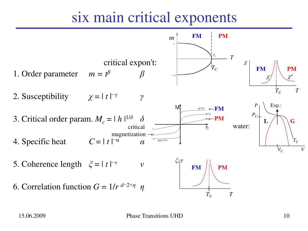
1. Specific Heat Exponent: $\alpha$

The exponent $\alpha$ describes the singularity in the specific heat $C$ at zero field ($h=0$).
$C(t)\sim |t{|}^{-\alpha }$
A positive $\alpha$ implies a divergence in the specific heat as $T\to T_c$. If $\alpha =0$, this often corresponds to a logarithmic divergence ($\ln |t|$). A negative $\alpha$ corresponds to a finite cusp at $T_c$.

2. Order Parameter Exponent: $\beta$

The exponent $\beta$ describes how the spontaneous order parameter (magnetization $m$) grows as the temperature is lowered below $T_c$. It's defined for $t<0$ and $h=0$.
$m(t)\sim (-t{)}^{\beta }$
This characterizes the shape of the coexistence curve near the critical point.

3. Susceptibility Exponent: $\gamma$

The exponent $\gamma$ describes the divergence of the susceptibility $\chi$ (the response of the order parameter to the field, $\chi =\partial m/\partial h$) at zero field.
$\chi (t)\sim |t{|}^{-\gamma }$
The divergence of $\chi$ reflects the fact that at criticality, an infinitesimally small field can produce a finite magnetization, indicating infinite sensitivity.

4. Critical Isotherm Exponent: $\delta$

The exponent $\delta$ describes the relationship between the order parameter and the field exactly at the critical temperature, $t=0$.
$m(h)\sim |h{|}^{1/\delta }(\text{at }t=0)$
This exponent characterizes the shape of the critical isotherm.

5. Correlation Length Exponent: $\nu$ (nu)

The exponent $\nu$ describes the divergence of the correlation length $\xi$, which is the characteristic length scale of order parameter fluctuations.
$\xi (t)\sim |t{|}^{-\nu }$
The divergence of $\xi$ is the most profound feature of a critical point: fluctuations become correlated over macroscopic distances. This is the origin of phenomena like critical opalescence.

6. Anomalous Dimension Exponent: $\eta$ (eta)

Finally, the exponent $\eta$ describes the power-law decay of the correlation function $G(r)=⟨\varphi (0)\varphi (r){⟩}_c$ precisely at the critical point ($t=0,h=0$).
$G(r)\sim \frac{1}{r^{d-2+\eta }}(\text{at }t=0,h=0)$
The term $d-2$ is the result from the simplest (Gaussian or Ornstein-Zernike) approximation. The exponent $\eta$ is thus a correction that measures the deviation from this simple behavior. In the language of field theory, which you'll appreciate from your QFT studies, $\eta$ is related to the anomalous dimension of the order parameter field $\varphi$, signifying how interactions modify its scaling properties.

---

This image provides an excellent visual summary of these six exponents and the physical behaviors they describe.

Test your understanding!

For the superfluid transition in helium, the specific heat exponent $\alpha$ is approximately -0.013. What does this negative value imply about the behavior of the specific heat at the transition temperature $T_{\lambda }$?

Show answer

A negative value of $\alpha$ means that the specific heat does not diverge. Since $|t{|}^{-\alpha }=|t{|}^{-(-0.013)}=|t{|}^{0.013}$, the function goes to zero as $t\to 0$. However, the specific heat itself is the sum of a regular part and this singular part. The singular part has a derivative that diverges as $|t{|}^{\alpha -1}=|t{|}^{-1.013}$. This results in a continuous function with an infinite slope at $T_c$, which is known as a cusp. So, the specific heat of helium is finite at the lambda point but has a very sharp peak with a vertical tangent.

Critical Exponents and Universality Classes

The values of these six exponents are the same for all systems within a given universality class. A universality class is determined by:

• The spatial dimension $d$.
• The symmetry of the order parameter (e.g., a scalar for Ising/liquid-gas, a 2D vector for XY model/superfluids, etc.).

The table below shows the exponent values for some important universality classes. Notice how they depend on dimension $d$, and how they differ significantly from the mean-field theory (MFT) predictions you have encountered. For $d=4$, the values match the MFT results for the Ising (${\varphi }^4$) model, which is consistent with the Ginzburg criterion establishing $d_c=4$ as the upper critical dimension.

This table makes the abstract concept of universality concrete. The fact that a 3D Ising magnet and a real 3D fluid share the same exponents (the $d=3$ column) is a profound statement about the organizing principles of nature at criticality.

Conclusion

Key Takeaways:

• The singular behavior of physical quantities near a critical point is described by a set of six standard critical exponents: $\alpha ,\beta ,\gamma ,\delta ,\nu ,\eta$.
• Each exponent characterizes a specific power-law behavior: $\alpha$ for specific heat, $\beta$ for the order parameter, $\gamma$ for susceptibility, $\delta$ for the critical isotherm, $\nu$ for the correlation length, and $\eta$ for the critical correlation function.
• The values of these exponents are universal, depending only on the spatial dimension and order parameter symmetry, not on the microscopic details of the system.
• Experimentally measured and accurately calculated exponents differ from mean-field predictions, highlighting the importance of fluctuations in $d\le 4$.

Preview of the Next Lesson:

Looking at the table of exponents, a natural question arises: are these six numbers all independent, or are they related to each other? For a given universality class, it seems we only need to specify a couple of them to know all the others.

In the next lesson, we will explore this very idea. We will introduce the scaling hypothesis, a powerful phenomenological assumption about the structure of the free energy near a critical point. We will see how this single hypothesis leads to a set of "scaling relations" that connect the different critical exponents, such as the Rushbrooke and Widom identities, thereby reducing the number of independent exponents from six to just two.