The Radon-Nikodym Derivative: A Generalized Density

In our last lesson, we introduced the Radon-Nikodym theorem, which guarantees that if a measure ν is absolutely continuous with respect to a σ-finite measure μ, a function f exists such that we can write ν(A) = ∫_A f dμ. We called this function the Radon-Nikodym derivative, dν/dμ, and saw its application in finance as the pricing kernel.

Today, we will delve into the interpretation of this derivative. The goal of this lesson is to understand why dν/dμ is considered a generalized density. We will connect this abstract concept to the familiar probability density functions (PDFs) from your statistics background and see how this new perspective provides a unified framework for describing probability distributions.

The Intuition: Density as a Ratio

At its heart, the concept of density is about a ratio: an amount of "stuff" per unit of "space". In physics, this is mass per unit volume. In probability, it's probability per unit of length (or area, or volume).

Consider a continuous random variable on the real line. The probability density function f(x) at a point x is not the probability at that point (which is zero). Instead, it gives us the rate at which probability accumulates around x. The probability of the variable falling in a tiny interval of width dx around x is approximately f(x)dx. This can be rearranged as f(x) ≈ P([x, x+dx]) / dx.

The Radon-Nikodym derivative formalizes and generalizes this very idea. Let's visualize it.

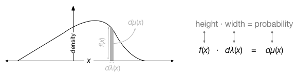
In this diagram, dμ(x) represents an infinitesimal element of a probability measure (the "stuff"), while dλ(x) represents an infinitesimal element of a reference measure, like length (the "space"). The density f(x) is the height that relates the two. The equation shown, f(x) = dμ(x) / dλ(x), is precisely the intuition behind the Radon-Nikodym derivative.

The following blog post explains this core idea very clearly.

As the post highlights, the probability measure μ is the crucial object. It encodes the actual probabilistic information. The density function f(x) is simply a convenient representation of μ with respect to a chosen reference measure λ. This is a subtle but powerful shift in perspective.

The Power of Changing the Reference Measure

If the density is just a representation relative to a reference measure, what happens if we change that reference? The underlying probability measure μ remains the same, but its density function will change. This is analogous to how the numerical value of a physical length changes depending on whether you measure it in meters or feet; the physical length itself is invariant.

This flexibility is one of the main strengths of the measure-theoretic approach. Sometimes, a distribution that has a complex density with respect to one reference measure might have a much simpler one with respect to another.

The example mentioned in the article, regarding the Logistic-Normal distribution becoming a simple multivariate Normal distribution under a change of measure, is a perfect illustration of this power. While we won't delve into that specific case, it underscores that the choice of reference measure is not just a theoretical curiosity but can have significant practical implications for simplifying models.

Unifying Discrete and Continuous Distributions

Now we arrive at the main payoff for your statistical understanding. The Radon-Nikodym framework elegantly unifies concepts that are typically taught separately in introductory statistics: probability density functions (PDFs) for continuous variables and probability mass functions (PMFs) for discrete variables.

From this new perspective, both are simply Radon-Nikodym derivatives, just with respect to different reference measures.

1. Probability Density Function (PDF): For a continuous random variable X on ℝ, the familiar PDF f(x) is the Radon-Nikodym derivative of its probability measure P with respect to the Lebesgue measure λ.

   $$f(x)=\frac{dP}{d\lambda }$$

   This means P(A) = ∫_A f(x) dλ(x) (or ∫_A f(x) dx), which is the standard definition you know.

2. Probability Mass Function (PMF): For a discrete random variable X taking values in, say, the integers ℤ, the PMF p(k) = P(X=k) is the Radon-Nikodym derivative of its probability measure P with respect to the counting measure c. The counting measure c(A) simply returns the number of points in the set A.

   $$p(k)=\frac{dP}{dc}$$

   With this, P(A) = ∫_A p(k) dc(k) = ∑_{k∈A} p(k), which again matches the standard definition.

The following video and notes reinforce this crucial point.

This unification is a key insight. It shows that PDFs and PMFs are not fundamentally different things; they are specific instances of a single, more general concept: a density relative to a chosen base measure.

Conclusion

In this lesson, we have unpacked the meaning of the Radon-Nikodym derivative, moving beyond its formal definition to an intuitive interpretation.

Here are the key takeaways:

• Generalized Density: The Radon-Nikodym derivative dν/dμ should be interpreted as the density of the measure ν relative to the reference measure μ. It generalizes the familiar concept of density by allowing the "ruler" (μ) to be something other than standard length or volume.
• The Primacy of the Measure: The probability measure itself is the fundamental object. A density function is merely a representation of that measure with respect to a chosen reference measure.
• A Unified Framework: This perspective elegantly unifies continuous and discrete distributions. A PDF is a density with respect to Lebesgue measure, while a PMF is a density with respect to counting measure.

We have now established that the Radon-Nikodym derivative is a generalized density. In the next lesson, we will formally state and confirm the most common special case: that a standard probability density function (PDF) is precisely the Radon-Nikodym derivative of a probability measure with respect to the Lebesgue measure. This will be the final piece of the Radon-Nikodym framework we need before we can deploy it to solve the paradox of conditioning on zero-probability events.