Radon-Nikodym Theorem and Probability Density Functions

Welcome to the final lesson of our first module. In our previous lessons, we built up the Radon-Nikodym framework, culminating in the interpretation of the Radon-Nikodym derivative as a generalized density. We saw that this powerful perspective unifies discrete and continuous distributions under a single conceptual umbrella.

Today, we will ground this abstract idea in a very concrete and familiar context. Our goal is to formally demonstrate that the standard probability density function (PDF) you have used throughout your studies in statistics and econometrics is a specific instance of a Radon-Nikodym derivative. Specifically, we will show that a PDF is the derivative of a probability measure with respect to the Lebesgue measure. This final step completes our foundational toolkit, preparing us to tackle the paradox of conditioning on zero-probability events in the next module.

From Calculus to Measure Theory

In your introductory probability and statistics courses, you defined the probability density function, $f(x)$, for a continuous random variable $X$ through its relationship with the cumulative distribution function (CDF), $F(x)$, as $f(x)=F^{\prime }(x)$. You then used it to calculate probabilities by integration:
$P(X\in A)={\int }_{A}f(x)dx$
From the perspective of your calculus courses, this is a Riemann integral. As we've discussed, measure theory provides a more powerful and general form of integration via the Lebesgue integral. A key first step is to recognize that the dx in the integral is not just a notational quirk; it signifies integration with respect to the Lebesgue measure, which we will denote by $\lambda$.

So, in measure-theoretic terms, the familiar equation above is written as:
$P(A)={\int }_{A}f(x)d\lambda (x)$
This equation involves two distinct measures on the real line:

1. The Probability Measure, $P$: This measure, induced by the random variable $X$, assigns a probability to any (Borel) set $A\subseteq \mathbb{R}$.
2. The Lebesgue Measure, $\lambda$: This is our reference measure, which assigns the standard notion of "length" to sets on the real line.

Now, look closely at the equation $P(A)={\int }_{A}f(x)d\lambda (x)$. This should look very familiar. It has the exact structure presented by the Radon-Nikodym theorem, which states that if a measure $P$ is absolutely continuous with respect to $\lambda$, there exists a function $f$ such that the equality holds.

The PDF as a Radon-Nikodym Derivative

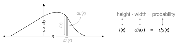
This observation leads directly to our main conclusion. The probability density function $f(x)$ is nothing more and nothing less than the Radon-Nikodym derivative of the probability measure $P$ with respect to the Lebesgue measure $\lambda$.
$f(x)=\frac{dP}{d\lambda }$
This formalizes the intuition we built in the last lesson. The PDF represents the "density" of probability measure relative to the standard "length" measure on the real line.

The following lecture notes from the University of Wisconsin-Madison make this connection explicit and formal.

The diagram below provides a powerful visual for this relationship.

To reinforce this point, the following video explains the Radon-Nikodym theorem by focusing on the Lebesgue measure as the reference.

The Prerequisite: Absolute Continuity

For the PDF to be the Radon-Nikodym derivative dP/dλ, the theorem requires that the probability measure $P$ be absolutely continuous with respect to the Lebesgue measure $\lambda$, written $P\ll \lambda$.

What does this mean? It means that any set with a Lebesgue measure of zero must also have a probability of zero.
$\lambda (A)=0⟹P(A)=0$
This is an intuitive condition for any random variable we would typically describe with a PDF. For example, any finite set of points $\{x_1,...,x_n\}$ has a length (Lebesgue measure) of zero. For a continuous random variable, the probability of it taking on any of those specific values is also zero. This condition essentially formalizes the idea that there are no "point masses" of probability; the probability is "smeared out" smoothly.

Extension to Higher Dimensions

This entire framework extends naturally to random vectors. For a pair of random variables $(X,Y)$, the joint probability measure $P_{XY}$ lives on ${\mathbb{R}}^2$. The corresponding reference measure is the two-dimensional Lebesgue measure, ${\lambda }_2$, which corresponds to area.

The joint PDF, $f(x,y)$, is then the Radon-Nikodym derivative of the joint probability measure with respect to the 2D Lebesgue measure:
$f(x,y)=\frac{d{P}_{XY}}{d{\lambda }_2}$
This means that for any region $A\subset {\mathbb{R}}^2$, the probability of $(X,Y)$ falling in that region is given by the integral of the joint PDF over that area:
$P_{XY}(A)={\iint }_{A}f(x,y)d{\lambda }_2(x,y)$

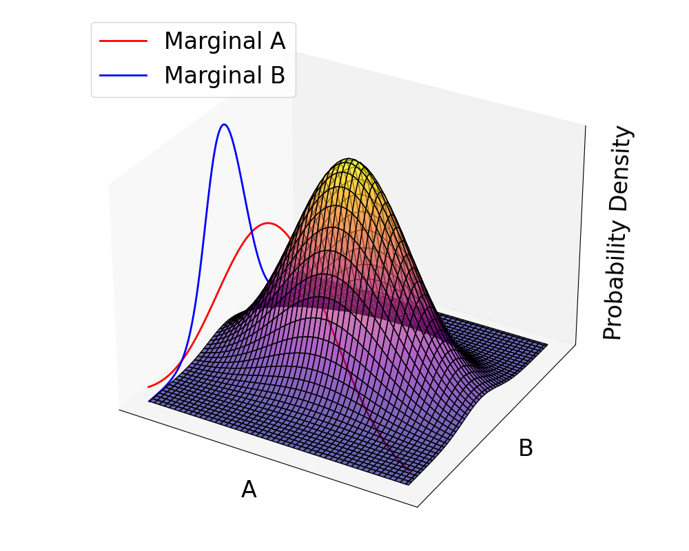
This multivariate view is precisely what we will need to analyze the bivariate normal distribution and resolve the conditioning paradox at the heart of your essay.

Conclusion

In this lesson, we have closed the loop, formally connecting the abstract Radon-Nikodym derivative to the familiar probability density function.

Key Takeaways:

• A standard PDF, $f(x)$, is the Radon-Nikodym derivative of its associated probability measure, $P$, with respect to the Lebesgue measure, $\lambda$. We write this as $f=dP/d\lambda$.
• This relationship is guaranteed by the Radon-Nikodym theorem, provided the probability measure is absolutely continuous with respect to the Lebesgue measure ($P\ll \lambda$).
• This concept extends to multiple dimensions, where a joint PDF is the Radon-Nikodym derivative with respect to the higher-dimensional Lebesgue measure (area, volume, etc.).

You have now completed the first module and have assembled all the conceptual machinery of the Radon-Nikodym framework needed for your essay. In the next module, "Resolving the Conditioning Paradox," we will deploy these tools to construct a rigorous definition of conditional expectation and show how it solves the problem of conditioning on events of probability zero.