Keynesian Consumption and the Expenditure Multiplier

Introduction

Welcome back! In our last lesson, we introduced the Aggregate Demand (AD) curve, defined its components as $AD=C+I+G+NX$, and explored the factors that cause the entire curve to shift. We established that changes in consumption, investment, government spending, or net exports can increase or decrease total demand in the economy at any given price level.

Today, we will delve deeper into the largest and most stable component of aggregate demand: Consumption (C). We'll explore the formal relationship between income and consumption, known as the Keynesian consumption function. This will then unlock a powerful concept in macroeconomics: the expenditure multiplier. You'll discover how an initial change in spending—say, by the government or a business—can have a magnified impact on the entire economy.

By the end of this lesson, you will be able to explain the Keynesian consumption function and calculate the total economic impact of a spending change using the expenditure multiplier. This understanding is crucial for analyzing how economic shocks and policy interventions ripple through the economy.

1. The Keynesian Consumption Function

The English economist John Maynard Keynes proposed that a household's consumption spending is directly and predictably related to its disposable income (the income left after paying taxes). This relationship forms the basis of the consumption function.

To get a clear understanding of the components and the mathematics, please watch the following video.

As the video explained, the consumption function can be expressed as:

$C=C_0+b\cdot Y_d$

Let's break down these components:

• $C$ is total consumption spending.
• $Y_d$ is disposable income (income after taxes).
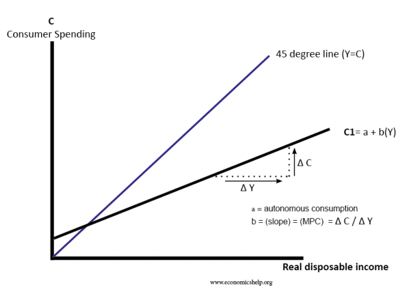
• $C_0$ is autonomous consumption: This is the amount of spending that occurs even when disposable income is zero. Think of it as spending on basic necessities, which might be financed by drawing down savings or borrowing. On a graph, this is the y-intercept of the consumption function.
• $b\cdot Y_d$ is induced consumption: This is the portion of spending that increases as disposable income increases.
• $b$ is the Marginal Propensity to Consume (MPC). It represents the fraction of an additional dollar of disposable income that is spent. For example, if your MPC is 0.8, you will spend 80 cents of every extra dollar you receive. The MPC is the slope of the consumption function: $MPC=\frac{\Delta C}{\Delta Y_d}$.

Since households can either spend or save their disposable income, we also have the Marginal Propensity to Save (MPS), which is the fraction of an additional dollar of disposable income that is saved. It follows that:

$MPC+MPS=1$

The image below provides a classic graphical representation of the consumption function.

2. The Expenditure Multiplier

Now that we understand that people spend a fraction of any new income they receive (the MPC), we can explore one of the most significant ideas in Keynesian economics: the expenditure multiplier.

The core idea is that an initial change in autonomous spending (e.g., government spending, investment) sets off a chain reaction that results in a much larger final change in national income (GDP).

The following video provides an excellent intuitive and mathematical explanation of this process.

The video demonstrates that an initial spending change creates a cascading effect. The process looks like this:

1. The government increases spending by $100 billion to build new roads.
2. This $100 billion becomes income for construction firms and their workers.
3. These workers and owners will spend a portion of this new income, determined by the MPC. If MPC = 0.8, they spend $80 billion on goods and services (food, clothing, etc.).
4. This $80 billion becomes income for grocers, retailers, and their employees.
5. They, in turn, spend a portion of it (0.8 * $80 billion = $64 billion), creating more income for others.

This process continues, with each round of spending being smaller than the last. The total change in GDP is the sum of this infinite geometric series, which simplifies to a neat formula for the simple expenditure multiplier:

$\text{Multiplier}=\frac{1}{1-MPC}\text{or}\text{Multiplier}=\frac{1}{MPS}$

The total change in GDP can then be calculated as:

$\Delta GDP=\text{Initial Change in Spending}\times \text{Multiplier}$

Notice that the multiplier's size depends entirely on the MPC. A higher MPC means a larger multiplier because less income "leaks" into savings at each round.

The diagram below shows this effect graphically. A relatively small upward shift in the aggregate expenditure line (from an increase in autonomous investment, $\Delta I$) leads to a much larger increase in the equilibrium level of output ($\Delta Y$).

3. A More Realistic Multiplier

The simple multiplier 1 / (1 - MPC) is a powerful concept, but it assumes the only "leakage" from the circular flow of income is savings. In the real world, income also leaks out in the form of taxes and spending on imports.

To get a more complete picture, I recommend reading the following text, which explains the multiplier effect in the context of a more realistic model.

As the reading describes, when you account for all leakages, the multiplier formula becomes:

$\text{Multiplier}=\frac{1}{\text{Sum of leakages}}=\frac{1}{\text{MPS}+\text{Tax Rate}+\text{MPI}}$

Where MPI is the Marginal Propensity to Import (the fraction of an additional dollar of income spent on imports). This more realistic multiplier will always be smaller than the simple multiplier, as there are more ways for spending power to leak out of the domestic economy in each round.

Practice Problem

Let's apply this. Assume an economy has an MPC of 0.75.

1. Simple case: The government increases spending by $50 billion. What is the total change in GDP?

   • First, find the MPS: $MPS=1-MPC=1-0.75=0.25$.
   • Next, calculate the multiplier: $\text{Multiplier}=\frac{1}{MPS}=\frac{1}{0.25}=4$.
   • Finally, find the total change in GDP: $\Delta GDP=\$50\text{ billion}\times 4=\$200\text{ billion}$.

2. More realistic case: Now assume, in addition to the MPC of 0.75, that the tax rate is 20% (0.2) and the MPI is 5% (0.05). What is the new multiplier and the total change in GDP from the same $50 billion spending increase?

   • The leakages are MPS (0.25), the tax rate (0.2), and MPI (0.05).
   • Sum of leakages = $0.25+0.20+0.05=0.50$.
   • New multiplier = $\frac{1}{0.50}=2$.
   • New total change in GDP = $\$50\text{ billion}\times 2=\$100\text{ billion}$.

As you can see, incorporating taxes and imports significantly reduces the impact of the multiplier.

Conclusion

In this lesson, we focused on the relationship between consumption and income, and the powerful ripple effect that changes in spending can have on the economy.

Key Takeaways:

• The Keynesian consumption function ($C=C_0+MPC\cdot Y_d$) formalizes the idea that consumption depends on a baseline level (autonomous consumption) and a level that changes with income (induced consumption).
• The Marginal Propensity to Consume (MPC) is the slope of this function and tells us the fraction of each new dollar of income that will be spent.
• The expenditure multiplier demonstrates that an initial change in autonomous spending leads to a larger final change in GDP.
• The size of the simple multiplier is determined by the formula $\frac{1}{1-MPC}$. A higher MPC leads to a larger multiplier.
• In a more realistic model, "leakages" like taxes and imports reduce the size of the multiplier.

Preview of the Next Lesson:

We have now explored Aggregate Demand in depth. To complete our model of the macroeconomy, we must turn to the supply side. In the next lesson, we will introduce the Aggregate Supply (AS) curve. We will examine why it has a different shape in the short run versus the long run and identify the factors that cause the AS curve to shift. Once we combine AD and AS, we will be able to analyze how the economy reaches an equilibrium level of output and prices, and how that equilibrium can be disrupted.