Recommended resources
The freely available resources this lesson will direct you to.
Introduction
Welcome to your second lesson in the module on "Aggregate Demand, Aggregate Supply, and Business Cycles." In our previous lesson, we described the recurrent, but irregular, fluctuations in economic activity known as the business cycle, identifying its four phases: expansion, peak, contraction, and trough.
Now, we move from describing these fluctuations to explaining them. To do this, we will build the primary tool of modern macroeconomics for analyzing the short run: the Aggregate Demand-Aggregate Supply (AD-AS) model. This lesson focuses on the first half of this model.
Our goal is to explain the components of the aggregate demand (AD) curve and identify factors that cause it to shift. By the end of this lesson, you will be able to:
- Define aggregate demand and its components.
- Explain why the aggregate demand curve is downward-sloping.
- Distinguish between a movement along the AD curve and a shift of the AD curve.
- Identify the key factors that cause the entire AD curve to shift.
This is the first building block in constructing a model that can explain why an economy might enter a recession or experience inflation.
1. Defining the Aggregate Demand Curve
In microeconomics, a demand curve shows the quantity of a single good that buyers are willing to purchase at different prices. Aggregate Demand (AD) scales this idea up to the entire economy. It represents the total demand for all domestically produced final goods and services at any given overall price level.
The AD curve is plotted on a graph with the price level (often measured by the GDP deflator or CPI) on the vertical axis and real GDP (total output) on the horizontal axis.
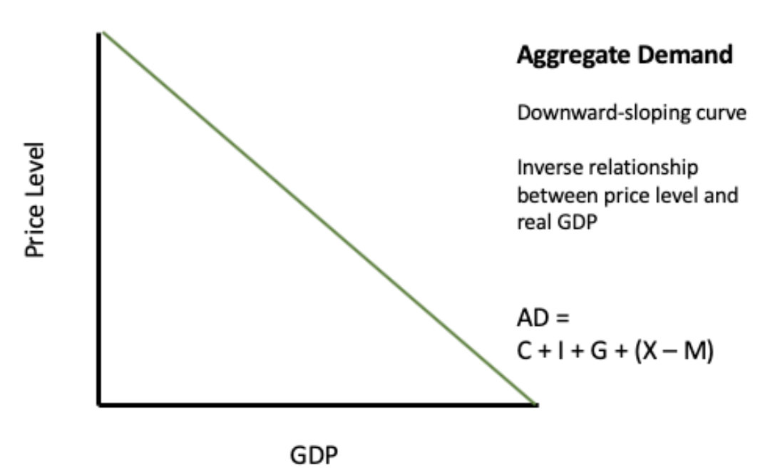
As you can see from the image, the formula for aggregate demand is identical to the expenditure approach for calculating GDP, which you learned in Module 8:
Where:
- C = Consumption spending by households
- I = Investment spending by firms
- G = Government spending on goods and services
- NX = Net Exports (Exports (X) - Imports (M))
Let's watch a brief video that introduces this concept.
Y1 4) Aggregate Demand - Shifts and the Downward Slope
This video from EconplusDal clearly defines aggregate demand as total expenditure in the economy and introduces its core components.
Watch the first 53 seconds of the video. Focus on the definition of aggregate demand and how it's measured by the C+I+G+(X-M) equation.
2. Why the Aggregate Demand Curve Slopes Downward
You'll notice the AD curve slopes downward, implying that as the overall price level falls, the total quantity of goods and services demanded increases. This seems intuitive, but the reasons are different from those for a single-good demand curve. For a single good, when its price falls, people substitute it for other, now relatively more expensive, goods. At the aggregate level, this substitution effect doesn't apply, because we are talking about a fall in the average price of all goods.
Instead, the downward slope of the AD curve is explained by three key macroeconomic effects.
Aggregate Demand- Macro Topic 3.1
Jacob Clifford's video offers a dynamic and clear explanation of the three effects that give the AD curve its negative slope.
Watch the segment from 01:34 to 03:19. Pay close attention to how a change in the price level affects consumption, investment, and net exports.
To solidify your understanding, let's review these three effects:
- The Wealth Effect: When the price level falls, the real value of money and other financial assets (like bonds) increases. A dollar you hold now has more purchasing power. This increase in real wealth makes consumers feel richer, and they tend to increase their consumption (C).
- The Interest-Rate Effect: A lower price level means households need less money to make their everyday purchases. They can save more. This increase in the supply of loanable funds in banks puts downward pressure on interest rates. Lower interest rates make borrowing cheaper for firms, encouraging more investment (I) in new capital. It also encourages household spending on interest-sensitive items like cars and houses.
- The International Trade Effect: If the price level in our country falls (while prices in other countries remain the same), our goods become cheaper and more attractive to foreign buyers. This leads to an increase in exports (X). At the same time, foreign goods become relatively more expensive for domestic consumers, leading to a decrease in imports (M). Both effects cause net exports (NX) to rise.
These three effects all show that a fall in the price level leads to an increase in the quantity of goods and services demanded. This is a movement along the AD curve. For a more detailed text explanation, especially on why the logic from microeconomics doesn't apply here, the following reading is highly recommended.
7.1 Aggregate Demand – BUS 400 Business Economics
This chapter from a business economics textbook provides a thorough explanation of the downward slope of the AD curve, including a crucial section differentiating it from a standard market demand curve.
Read the section titled 'The Slope of the Aggregate Demand Curve'. Pay special attention to the paragraphs explaining why you cannot apply the reasoning from individual markets (substitution and income effects) to the aggregate demand curve. This is a key conceptual point.
3. Shifts in the Aggregate Demand Curve
A movement along the AD curve is caused only by a change in the overall price level. A shift of the AD curve, however, occurs when the total quantity of goods and services demanded changes at every price level.
This happens when one of the components of aggregate demand—C, I, G, or NX—changes for a reason other than a change in the price level.
- An increase in AD is a shift to the right.
- A decrease in AD is a shift to the left.
The following video provides excellent, practical examples of events that shift the AD curve.
Aggregate Demand- Macro Topic 3.1
Let's return to Jacob Clifford's video, where he uses six scenarios to test your understanding of what causes the AD curve to shift.
Watch from 03:19 to 05:40. For each of the six scenarios presented, try to predict the outcome yourself before the explanation is given. This is a great way to actively test your knowledge.
As the video demonstrated, any event that changes C, I, G, or NX (independently of the price level) is an AD shifter. Let's organize these shifters by component.
Shifts in Aggregate Demand | Macroeconomics - Lumen Learning
This text from Lumen Learning offers a structured overview of the shifters, separating them into changes in consumer/firm behavior and changes in government policy. It also includes an important clarification on the role of imports.
Read through the following sections to get a comprehensive view of the shifters: 'Shifts in Aggregate Demand': For the definition of positive and negative demand shocks. 'Do Imports Diminish Aggregate Demand?': This is a very useful section that clarifies a common misconception about the role of imports (M) in the AD formula. 'How Changes by Consumers and Firms Can Affect AD': Focus on how consumer and business confidence impact C and I. 'How Government Macroeconomic Policy Choices Can Shift AD': Understand how government spending (G) and taxes (which affect C and I) are key policy tools. 'Government Policy Options': Briefly notes the role of monetary policy, which we will cover later.
The image below provides a great summary of the key shifters and how they affect the AD curve.

Here is a summary table of the primary AD shifters:
| Component | Increases AD (Shifts Right) | Decreases AD (Shifts Left) |
|---|---|---|
| C | ↑ Consumer confidence, ↓ Taxes, ↑ Transfer payments | ↓ Consumer confidence, ↑ Taxes, ↓ Transfer payments |
| I | ↑ Business confidence, ↓ Interest rates, Tax incentives | ↓ Business confidence, ↑ Interest rates |
| G | ↑ Government purchases (e.g., defense, infrastructure) | ↓ Government purchases |
| NX | ↑ Foreign income, Depreciation of domestic currency | ↓ Foreign income, Appreciation of domestic currency |
Conclusion
In this lesson, we have constructed the first half of the essential AD-AS model. We moved from simply measuring the economy with GDP to modeling the total demand for all goods and services within that economy.
Key Takeaways:
- Aggregate Demand (AD) is the total spending on an economy's goods and services, given by the formula .
- The AD curve slopes downward due to the wealth effect, the interest-rate effect, and the international trade effect. A change in the price level causes a movement along the curve.
- The AD curve shifts when a component (C, I, G, or NX) changes for a reason other than a change in the price level.
- Key shifters include changes in consumer/business confidence, government fiscal policy (spending and taxes), and international factors (foreign income and exchange rates).
Preview of the Next Lesson:
Understanding demand is only half the story. The behavior of the economy also depends on the willingness and ability of firms to produce goods and services. In the next lesson, we will build the second half of our model: the Aggregate Supply (AS) curve. We will explore why it has different shapes in the short run and the long run, and identify the factors that cause it to shift. Once we have both AD and AS, we can put them together to see how the economy arrives at an equilibrium level of output and prices.