Inference Batching Strategies: Latency & Throughput Impacts

Introduction

Welcome to the second lesson on "Inference at Scale." In our last session, we established the fundamental differences between training and inference workloads. We concluded that while training prioritizes raw throughput to minimize time-to-solution, inference is a delicate balancing act between latency, throughput, and cost. A key insight was that for many modern AI models, particularly LLMs, inference is profoundly memory-bandwidth bound, meaning the GPU often sits idle, waiting for data.

This lesson builds directly on that foundation. If inference is inefficient for a single request, how can we improve utilization and serve more users cost-effectively? The answer lies in batching. This is perhaps the most fundamental software optimization for any inference system.

Today, we will address the learning outcome: Describe inference batching strategies (static, dynamic, and continuous) and their impact on latency and throughput. We will explore a taxonomy of these strategies, analyzing their mechanisms, the inefficiencies they introduce or solve, and the critical design trade-offs they present.

The Rationale for Batching

Before diving into different strategies, let's solidify why batching is necessary. As we discussed, a single inference request, especially during the token-by-token generation (decode) phase, involves matrix-vector operations that are too small to saturate the massive parallel compute capabilities of a GPU. The bottleneck becomes loading the model's weights from high-bandwidth memory (HBM).

Batching addresses this by grouping multiple requests together. Instead of performing many small, memory-bound operations, the system can perform one large matrix-matrix multiplication. This increases the amount of computation per byte of data loaded (arithmetic intensity), allowing the cost of fetching model weights to be amortized across many requests. The result is a significant boost in overall system throughput and hardware utilization.

To understand the nuances of batching, it's crucial to recognize that an LLM inference request has two distinct computational phases, a concept we will build upon throughout this lesson.

A Taxonomy of Batching Strategies

The evolution from simple to sophisticated batching methods reflects a deeper understanding of the workload's unique characteristics. Let's trace this evolution from static to dynamic, and finally to continuous batching.

1. Static Batching: The Rigid Foundation

Static batching is the most basic approach. The inference server waits until a fixed number of requests have arrived, groups them into a batch, and processes them. Crucially, the system must wait for every single request in the batch to finish generating its complete output before it can start processing the next batch.

This introduces two major sources of inefficiency:

1. Padding: To be processed as a single tensor, all sequences in the batch must have the same length. Shorter sequences are "padded" with extra, meaningless tokens, forcing the GPU to waste compute cycles on them.
2. Head-of-Line (HOL) Blocking: The entire batch's completion time is determined by the longest-running request. If one request asks for a long summary and the others are simple questions, the GPU resources for the completed requests sit idle, waiting for the "straggler." This leads to a sawtooth pattern of GPU utilization and poor overall throughput.

The following video provides a clear, animated illustration of this inefficiency.

Despite its flaws, static batching can be effective for offline, bulk-processing tasks where all requests are very similar in length and latency is not a concern.

2. Dynamic Batching: A Small Step Forward

Dynamic batching introduces a slight improvement. Instead of only waiting for a fixed batch size, the server forms a batch when either the size threshold is met OR a time window expires.

This primarily helps reduce latency during periods of low traffic, as the first few requests don't have to wait indefinitely for the batch to fill. However, once the batch is created and sent to the GPU, it is processed identically to a static batch. It still suffers from the exact same Head-of-Line blocking and padding inefficiencies. It improves when a batch starts, but not how the batch is processed.

3. Continuous Batching: The Paradigm Shift

Continuous batching, also known as iteration-level batching, fundamentally rethinks the problem. It moves from a coarse-grained, request-level scheduling model to a fine-grained, iteration-level one.

The core idea is to decouple the lifecycles of individual requests. Instead of managing static "batches," the system maintains a dynamic pool of active requests.

The process works as a continuous loop:

1. Forward Pass: At each step, the system performs one forward pass for all requests currently in the active pool, generating one new token for each.
2. Completion Check: After the pass, the system checks if any request has generated its end-of-sequence token.
3. Immediate Eviction: Any completed requests are immediately removed from the pool, and their resources (especially their KV cache memory) are freed.
4. Admission: The system checks for available capacity and admits new requests from a waiting queue into the pool.
5. Repeat: The loop continues.

This mechanism completely eliminates Head-of-Line blocking. A short request is never forced to wait for a long one. Freed resources are immediately backfilled with new work, leading to consistently high GPU utilization and dramatically higher throughput.

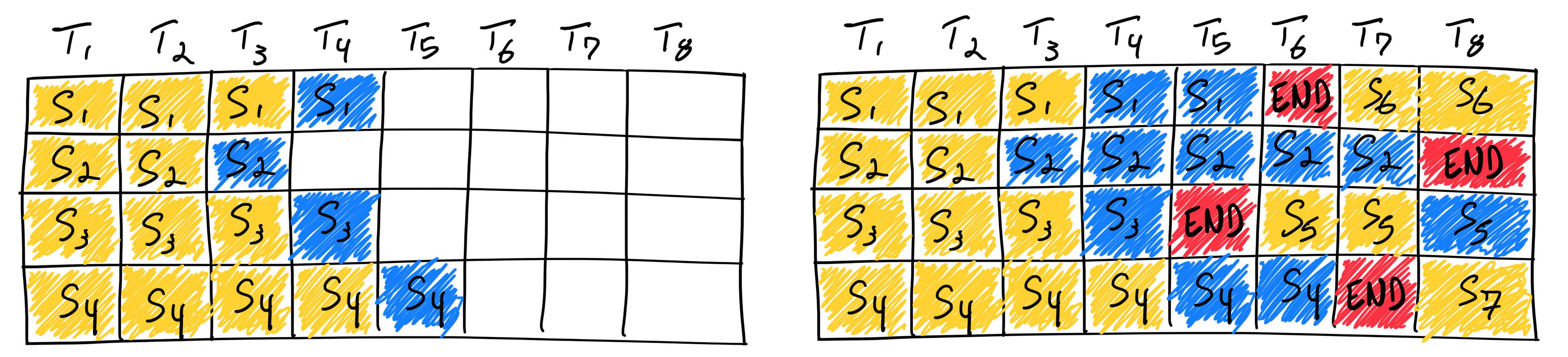
Let's watch a visualization of this much more efficient process.

The blog post we read earlier provides a comprehensive summary of these three strategies.

The Prefill-Decode Trade-off: A Deeper Look

For your background, it's worth digging into a more subtle and advanced aspect of continuous batching. While we've treated "continuous batching" as a single concept, modern systems like vLLM or TensorRT-LLM implement it with a specific scheduling policy that creates its own important trade-off.

Recall the prefill (processing the prompt) and decode (generating tokens one-by-one) phases. The prefill phase for a long prompt can be very compute-intensive and take a significant amount of time, whereas a decode step is very fast. What should a serving system do when a new request arrives (requiring a long prefill) while other requests are in their fast decode phase?

Many popular systems use a prefill-prioritizing schedule. They will pause the decoding of ongoing requests to run the prefill for the new request. This is done because it gets the new request into the decoding pool quickly, maximizing the batch size for subsequent decode steps and thus maximizing overall system throughput.

However, this comes at a cost: the ongoing requests experience a "generation stall." Their users see a sudden pause in the stream of tokens, which significantly increases the tail latency for the Time-Between-Tokens (TBT) metric. This creates a fundamental trade-off between maximizing throughput and providing low, consistent latency.

The academic paper below, which introduces a system called Sarathi-Serve, provides a rigorous analysis of this problem.

To mitigate this, advanced techniques like chunked prefill have been developed. Instead of running a long prefill operation in one go, the system breaks it into smaller chunks and interleaves them with the decode steps of other requests. This smooths out the computation, preventing long stalls and improving latency, while still working to increase batch size.

Conclusion

In this lesson, we dissected the evolution of batching strategies for LLM inference, moving from inefficient static methods to highly effective continuous batching.

Key Takeaways:

• Batching is Essential: It's the primary technique to overcome the memory-bound nature of single-request inference and improve GPU utilization and throughput.
• Static/Dynamic Batching Suffer from HOL Blocking: By treating a batch as an atomic unit, these request-level strategies lead to significant GPU idle time and wasted computation due to padding.
• Continuous Batching Eliminates HOL Blocking: By operating at an iteration-level, it decouples request lifecycles, allowing requests to join and leave a dynamic pool at any step. This maximizes resource utilization and throughput.
• The Prefill-Decode Scheduling Trade-off: Even within continuous batching, a critical design choice exists. Prioritizing prefill operations boosts throughput but can cause "generation stalls" that harm latency (TBT). Advanced techniques like chunked prefill aim to mitigate this trade-off.

Understanding these different batching strategies and their associated trade-offs is crucial for designing and operating a high-performance, cost-effective inference service.

Preview of the Next Lesson:

Batching is a powerful scheduling optimization. In our next lesson, we will explore a powerful model optimization technique that also attacks the memory bottleneck: model quantization. We will cover the learning outcome: Explain model quantization (e.g., INT8/INT4) and its effect on performance, memory usage, and accuracy. This will show us how reducing the numerical precision of the model itself can further reduce memory pressure and accelerate inference.