Recommended resources
The freely available resources this lesson will direct you to.
- AI Inference: The Secret to AI's Superpowerswww.youtube.com
- Exploring the Latency/Throughput & Cost Space for LLM Inference // Timothée Lacroix // CTO Mistralwww.youtube.com
- AI inference crisis: Google engineers on why network latency and ...www.sdxcentral.com
- [PDF] AI Hardware Accelerators: Architecture Trade-offs, Performance ...ijisae.org
Introduction
Welcome to the first lesson in our module on "Inference at Scale." In previous modules, we've focused heavily on optimizing the performance of large-scale AI model training. We've explored everything from parallelizing computations on a single GPU to orchestrating massive distributed jobs with techniques like topology-aware task placement.
Now, we pivot our attention to the second, and arguably more economically significant, phase of an AI model's lifecycle: inference. This is the process of using a trained model to make predictions on new, unseen data. While training and inference are two sides of the same coin, their system requirements, performance goals, and optimization strategies are profoundly different.
In this lesson, we will directly address the learning outcome: Contrast the system requirements and optimization goals of training vs. inference workloads (latency, throughput, and cost). Understanding this distinction is fundamental to designing efficient and scalable AI systems, as a system optimized for training is often poorly suited for production inference, and vice-versa.
What are Training and Inference?
At a high level, training is the "learning" phase, while inference is the "doing" phase. Let's start with a clear definition of these two stages.
AI Inference: The Secret to AI's Superpowers
This video from IBM Technology provides a concise overview of AI training and inference, using a simple spam detection model as an example. It clearly explains the core purpose of each stage.
Please watch the video from the beginning to 4:56. Focus on the distinction between how a model learns patterns from a large, labeled dataset (training) and how it applies those learned patterns to make predictions on new data (inference).
As the video illustrates, training involves an iterative process of feeding a model vast amounts of data, calculating errors, and adjusting model weights via backpropagation. It's a computationally massive, offline process. Inference, by contrast, is a single forward pass through the network to generate a result. It often needs to happen in real-time.
This fundamental difference in the workload leads to a completely different set of optimization priorities.
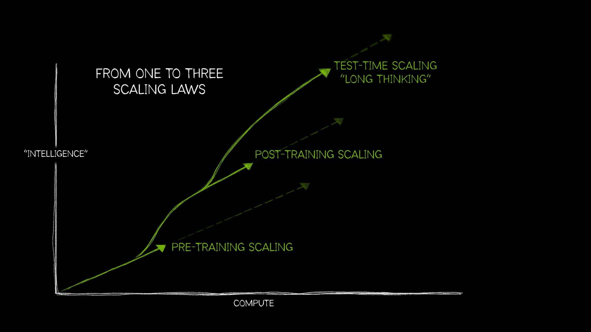
The Core Optimization Triangle: Latency, Throughput, and Cost
The primary goals of any system can be distilled into a trade-off between latency, throughput, and cost. How we prioritize these three metrics is the key differentiator between training and inference systems.
For Training:
- Primary Goal: Minimize the total time-to-train.
- Key Metric: Throughput. This is measured in terms of how much data can be processed per unit of time (e.g., samples/second, tokens/second). Higher throughput means the model sees the entire dataset faster, and the training job finishes sooner.
- Latency: The latency of individual training steps is secondary. As long as the pipeline is full and the GPUs are saturated, a higher latency per step is acceptable if it leads to a larger batch size and thus higher overall throughput.
- Cost: Training is a massive, but often infrequent, capital expenditure (CapEx). The focus is on acquiring powerful hardware (many high-end GPUs, fast interconnects) to reduce the training time, as the cost of engineering time and time-to-market often outweighs the hardware cost.
For Inference:
- Primary Goal: Serve user requests with a good experience at a minimal cost.
- Key Metrics: A balance of Latency and Throughput.
- Latency is often critical for user experience. For a chatbot, this means low time-to-first-token so the user sees a quick response, and low time-per-token so the text streams smoothly. For a recommendation engine, it's the end-to-end time to return a result.
- Throughput is measured in queries-per-second (QPS). The system must handle a certain load of concurrent users. The goal is to maximize QPS while keeping latency below a specific threshold (a Service Level Objective, or SLO).
- Cost: Inference is an ongoing operational expenditure (OpEx) that scales directly with usage. The cost-per-inference is a critical business metric.
This cost distinction is perhaps the most crucial. While training a large model is expensive, deploying it to millions of users can be far more so over its lifetime.
AI Inference: The Secret to AI's Superpowers
Let's return to the IBM video, which makes a powerful point about the economics of inference.
Watch the segment from 4:56 to 7:30. Pay close attention to the claim that inference can account for up to 90% of an AI model's lifetime cost and carbon footprint. This highlights why optimizing inference is so critical from a business and operational perspective.
To formalize the inference metrics, especially in the context of Large Language Models (LLMs), the CTO of Mistral AI provides a crisp definition.
Exploring the Latency/Throughput & Cost Space for LLM Inference // Timothée Lacroix // CTO Mistral
This clip from a talk by Timothée Lacroix, CTO of Mistral AI, precisely defines the key metrics for LLM inference.
Watch this short segment from 3:25 to 4:11. Note how he separates throughput (for batch jobs or user capacity) from latency (for user experience) and adds cost as the third dimension.
The following diagram provides a fantastic summary of how these differing requirements influence the choice of hardware and system design.

How Workload Differences Drive System Design
The distinct goals of training and inference lead to fundamentally different bottlenecks and, therefore, different system architectures.
A key academic paper on AI accelerators provides an excellent summary of these architectural requirements. The table below, adapted from the paper, quantifies the differences.
| Requirement | Training | Inference (Data Center) | Inference (Edge) |
|---|---|---|---|
| Numerical Precision | FP32 / FP16 | INT8 / FP16 | INT8 / INT4 |
| Batch Size | Large (128 - 4096+) | Small-to-Medium (1 - 128) | Single-digit (1 - 8) |
| Latency Target | Relaxed (seconds/minutes) | Strict (<100ms) | Very Strict (<10ms) |
| Memory Capacity | Very High (e.g., 80GB+) | Medium (e.g., 16-24GB) | Low (e.g., 1-4GB) |
| Power Budget | High (300-700W per GPU) | Medium (75-250W) | Very Low (5-15W) |
| Cost Priority | Medium (Time is primary) | High | Critical |
Source: Adapted from Table III in "[PDF] AI Hardware Accelerators: Architecture Trade-offs, Performance... " (Resource LINK)
Let's dissect this, focusing on the data center context that is most relevant to our course.
The Training System: Optimized for Throughput and Flexibility
- Workload: Involves both a forward pass and a backward pass (backpropagation), plus gradient updates. It's computationally much heavier than inference.
- Hardware: Relies on the most powerful, general-purpose GPUs (e.g., NVIDIA H100). These offer massive floating-point operation throughput (FLOPS), large high-bandwidth memory (HBM) to hold model parameters, activations, and gradients for large batches, and are fully programmable via frameworks like CUDA. Flexibility is paramount because research and model architectures evolve rapidly.
- Bottleneck: Can be compute-bound for models with high arithmetic intensity, memory-bandwidth-bound when loading weights, or, as we've seen, network-bound in large-scale distributed runs. The system is a delicate balance of all three.
The Inference System: Optimized for Latency and Efficiency
- Workload: A single, feed-forward pass. The model architecture is fixed. This stability allows for aggressive, specialized optimizations.
- Hardware: A diverse ecosystem exists. While GPUs are still common, specialized ASICs (Application-Specific Integrated Circuits) like Google's TPUs or AWS's Inferentia chips are designed specifically for inference. They strip out unnecessary components (like graphics-rendering hardware or high-precision units needed for training), leading to dramatic improvements in performance-per-watt and performance-per-dollar.
- Bottleneck: For many workloads, especially LLMs, the bottleneck is famously memory bandwidth, not compute.
The idea that inference is memory-bound, not compute-bound, is one of the most important concepts in modern AI system design. Let's explore why.
AI inference crisis: Google engineers on why network latency and memory trump compute
This article, titled 'AI inference crisis', features insights from Google engineers David Patterson and Xiaoyu Ma. It argues compellingly that the core challenges for LLM inference are memory and networking, not a lack of compute power.
Please read the introduction and the sections 'Memory hits a wall' and 'Latency: The network bottleneck'. Focus on these key arguments: Why the sequential, token-by-token 'decode' phase of LLM inference is 'inherently sequential' and thus memory-bound. The growing gap between compute (FLOPS) growth and memory bandwidth growth. The crucial difference in networking needs: training requires high bandwidth for large messages, while inference requires low latency for frequent, small messages.
The Mistral CTO's talk provides a quantitative backbone to this argument. He introduces the concept of an "ideal batch size" (B*) where a system transitions from being memory-bound to compute-bound.
Exploring the Latency/Throughput & Cost Space for LLM Inference // Timothée Lacroix // CTO Mistral
Let's revisit the Mistral talk for a more technical explanation of the memory-bound nature of LLM inference.
Watch the segment from 4:11 to 9:46. You don't need to memorize the formulas, but focus on the conceptual graph he draws. The flat part of the latency curve is the memory-bound regime, where the GPU is waiting on data to be loaded. The time is dominated by Model Size / Memory Bandwidth. The rising part is the compute-bound regime. He calculates that the ideal batch size (B*) to become compute-bound is very large (e.g., 400), but practical memory constraints (especially for the KV cache) limit the actual batch size to be much smaller (e.g., 5 to 33). The conclusion is that for most practical purposes, LLM decoding is 'severely memory bandwidth bound.'
This analysis is critical. It explains why simply adding more compute (TFLOPS) to an inference accelerator may yield diminishing returns if not accompanied by a proportional increase in memory bandwidth—a trend that is not currently happening. It also motivates many of the software optimizations we will discuss in future lessons, such as quantization and operator fusion, which are designed specifically to reduce the memory footprint and bandwidth pressure.
Conclusion
In this lesson, we have established the fundamental dichotomy between AI training and inference. Mistaking one for the other is a common and costly error in system design.
Key Takeaways:
- Divergent Goals: Training prioritizes throughput to minimize time-to-solution, accepting high upfront CapEx. Inference balances latency and throughput to optimize user experience and cost-per-query, focusing on low ongoing OpEx.
- Different Workloads: Training is a complex, iterative process involving both forward and backward passes. Inference is a simpler, single forward pass on a fixed model.
- Contrasting Bottlenecks: While training performance is a balance of compute, memory, and network, LLM inference is notoriously memory-bandwidth-bound and network-latency-sensitive due to its sequential, autoregressive nature.
- Hardware Specialization: The flexibility of programmable GPUs is ideal for evolving training workloads. The stability of inference workloads enables the use of highly efficient, specialized hardware like ASICs that provide superior performance-per-watt and performance-per-dollar.
Ultimately, designing a system for training is about building a powerful, flexible engine for research and development. Designing for inference is about engineering a highly-optimized, cost-efficient production service.
Preview of the Next Lesson:
Now that we understand the critical importance of balancing latency and throughput for inference, we will dive into one of the most powerful software techniques for managing this trade-off. In the next lesson, we will cover the learning outcome: "Describe inference batching strategies (static, dynamic, and continuous) and their impact on latency and throughput." We'll see how grouping requests together can dramatically improve system efficiency, but at a potential cost to latency.