Recommended resources
The freely available resources this lesson will direct you to.
Hello! Last lesson, you used a correlated subquery to compare each paid order with the average paid order in its own region. Today you’ll calculate that regional benchmark beside each order with OVER and PARTITION BY. You’ll also use the same pattern for regional totals and each order’s share of that total—calculations that preserve the order-level detail a data analyst often needs.
Keep the order, add the group metric
Suppose you need a regional sales total. GROUP BY region gives you one row per region, but no individual order rows. A window function can put the regional total beside each order without collapsing those rows.
Watch the short comparison and syntax demonstration in SQL Window Functions in 10 Minutes by Colt Steele. Its examples use departments and salaries; we’ll apply the same logic to orders and regions.
SQL Window Functions in 10 Minutes
Watch SQL Window Functions in 10 Minutes by Colt Steele for a visual comparison of grouped results and row-preserving window calculations.
Start with the comparison between GROUP BY and a department average beside each employee. Then watch OVER() for a calculation across all rows, followed by PARTITION BY for separate departmental calculations. Focus on what happens to the number of output rows.
The following diagram shows the same distinction with departmental totals.
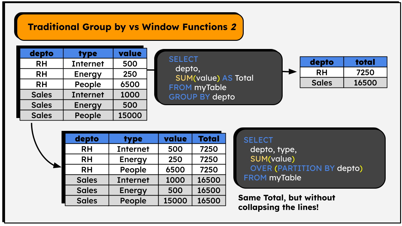
The PostgreSQL syntax is:
aggregate_function(column) OVER (PARTITION BY group_column)
OVER makes the aggregate a window calculation. PARTITION BY defines which rows share a calculation; it does not change the output to one row per partition. With OVER () and no partition, the calculation covers all rows available to the window function.
For an authoritative explanation of which rows those are, read the indicated passages of PostgreSQL’s Window Functions tutorial. Leave its ranking and running-sum examples for later lessons.
Documentation: 18: 3.5. Window Functions
Read PostgreSQL’s Window Functions tutorial to connect the syntax to row preservation, partition membership, and query filtering.
In Section 3.5, “Window Functions,” begin with the opening paragraph and its key contrast. Just below the employee-salary example, read the explanation of OVER and PARTITION BY. Farther down, after the row_number example, read the input rules. Finally, after the ordered-sum example, read the placement rule.
Calculate benchmarks beside paid orders
We’ll use the orders_stage data from the previous lesson. If that temporary table is still available in your PostgreSQL session, skip this setup. Otherwise, recreate it:
CREATE TEMP TABLE orders_stage (
    order_id integer PRIMARY KEY,
    region text,
    ordered_on date,
    status text,
    amount numeric(10, 2)
);

INSERT INTO orders_stage
    (order_id, region, ordered_on, status, amount)
VALUES
    (1, 'North', '2025-01-01', 'paid',      100.00),
    (2, 'North', '2025-01-01', 'paid',       50.00),
    (3, 'North', '2025-01-02', 'cancelled',  40.00),
    (4, 'North', '2025-01-02', 'pending',    70.00),
    (5, 'South', '2025-01-01', 'paid',       80.00),
    (6, 'South', '2025-01-01', 'cancelled',  20.00),
    (7, 'South', '2025-01-02', 'paid',        NULL),
    (8, 'South', '2025-01-03', 'pending',    30.00),
    (9, 'South', '2025-01-03', NULL,         10.00);
The business question is: For each paid order, what is the overall paid-order average, its region’s paid-order average, and its region’s paid amount? Each window expression answers a different part:
SELECT
    order_id,
    region,
    amount,
    ROUND(AVG(amount) OVER (), 2) AS all_paid_avg,
    ROUND(AVG(amount) OVER (PARTITION BY region), 2)
        AS region_paid_avg,
    SUM(amount) OVER (PARTITION BY region)
        AS region_paid_total
FROM orders_stage
WHERE status = 'paid'
ORDER BY region, order_id;
| order_id | region | amount | all_paid_avg | region_paid_avg | region_paid_total |
|---|---|---|---|---|---|
| 1 | North | 100.00 | 76.67 | 75.00 | 150.00 |
| 2 | North | 50.00 | 76.67 | 75.00 | 150.00 |
| 5 | South | 80.00 | 76.67 | 80.00 | 80.00 |
| 7 | South | NULL | 76.67 | 80.00 | 80.00 |
Read across order 1. Its amount is 100; the average of all recorded paid amounts is about 76.67; the average of North’s paid amounts is 75; and North’s paid amount totals 150. Order 2 gets the same North benchmarks because it belongs to the same partition, but it remains a separate output row.
This is the same regional average you calculated with a correlated subquery last lesson. The change is in how you express it: rather than referring to an outer order’s region from an inner query, PARTITION BY region supplies the matching group to each output row. The final ORDER BY region, order_id merely sorts the displayed result; it does not define the window.
Decide which rows belong in each calculation
A window function sees the rows remaining after this query’s WHERE filter. Here, WHERE status = 'paid' removes cancelled, pending, and unknown-status orders before any of the displayed averages or totals are calculated. Taking that condition away would change the business metric, not just add more output rows.
Missing amounts require another decision. Order 7 is still a paid order and still appears, but AVG(amount) and SUM(amount) ignore its NULL amount. That is why South’s paid average and total are both 80. Compare two counts to see the distinction:
SELECT
    order_id,
    region,
    amount,
    COUNT(*) OVER (PARTITION BY region) AS paid_orders,
    COUNT(amount) OVER (PARTITION BY region)
        AS paid_orders_with_amount
FROM orders_stage
WHERE status = 'paid'
ORDER BY region, order_id;
Both South rows display paid_orders = 2, but paid_orders_with_amount = 1. The first counts paid-order rows; the second counts paid orders with a non-null amount. Neither is automatically the “right” count—the metric definition determines which you need.
A partition can also use more than one column. For example, on the unfiltered table, COUNT(*) OVER (PARTITION BY region, status) would count orders for each region-and-status combination while leaving individual orders visible. Orders 5 and 7 would each show 2 for South and paid; South’s cancelled order would show 1. Choosing partition columns is therefore choosing the level at which the benchmark is calculated.
Build a row-level contribution metric
A common analytical question is what percentage of its region’s recorded paid amount did each order contribute? The numerator is the order amount; the denominator is the regional total repeated beside that order:
SELECT
    order_id,
    region,
    amount,
    ROUND(
        100.0 * amount
        / NULLIF(SUM(amount) OVER (PARTITION BY region), 0),
        1
    ) AS pct_of_region_paid_amount
FROM orders_stage
WHERE status = 'paid'
ORDER BY region, order_id;
| order_id | region | amount | pct_of_region_paid_amount |
|---|---|---|---|
| 1 | North | 100.00 | 66.7 |
| 2 | North | 50.00 | 33.3 |
| 5 | South | 80.00 | 100.0 |
| 7 | South | NULL | NULL |
North’s percentages use 150 as their shared denominator. South’s recorded paid amount totals 80, so order 5 accounts for 100% of it; that does not mean South had only one paid order. Order 7’s contribution is unknown because its amount is missing. NULLIF prevents division by zero if a region’s recorded amounts sum to zero.
The pattern is useful whenever a report needs both a detailed record and its group context: a transaction and regional sales, for example, or an item and its category’s total.
Filter after calculating a window value
You may want to return only paid orders above their regional paid average, as you did last lesson. The window expression cannot go directly in this query’s WHERE: PostgreSQL evaluates that filter before window calculations. Put the calculation in an inner query, then filter its result in an outer query:
SELECT
    order_id,
    region,
    amount,
    region_paid_avg
FROM (
    SELECT
        order_id,
        region,
        amount,
        AVG(amount) OVER (PARTITION BY region)
            AS region_paid_avg
    FROM orders_stage
    WHERE status = 'paid'
) AS paid_with_avg
WHERE amount > region_paid_avg
ORDER BY order_id;
| order_id | region | amount | region_paid_avg |
|---|---|---|---|
| 1 | North | 100.00 | 75.00 |
The inner query establishes the paid-order population and calculates each region’s average. The outer query then keeps orders above that already-calculated value. South’s order 5 equals its regional average rather than exceeding it, while order 7’s missing amount cannot pass the comparison.
Key takeaways
OVER () calculates across the available rows without collapsing them; OVER (PARTITION BY region) calculates separately for each region while retaining one output row per input row. Filters determine which rows participate before the window calculation, and aggregate functions treat missing values according to their usual rules. To filter on a window result, calculate it in an inner query first.
Next, you’ll add ordering inside OVER to assign positions within groups using ROW_NUMBER, RANK, and DENSE_RANK.