AllReduce for Gradient Synchronization

Introduction

Welcome to the next lesson in our module on multi-GPU communication. In our previous session, we explored how collective communication libraries like NCCL provide a vital abstraction layer. We saw that by offering a high-level API for operations like Broadcast and AllReduce, NCCL shields developers from the immense complexity of programming directly against hardware interconnects like NVLink and InfiniBand. We learned that NCCL acts as a "dataflow compiler," intelligently choosing the best transport, protocol, and algorithm at runtime to maximize performance.

This lesson zooms in on the single most critical collective operation for training large-scale AI models: AllReduce. The learning outcome for this lesson is to describe the AllReduce collective operation and its function in synchronizing gradients for data-parallel training.

We will cover:

• The precise definition of the AllReduce operation.
• Its essential role within the data-parallel training paradigm for ensuring model consistency.
• How AllReduce is used to aggregate gradients calculated across multiple GPUs.
• A high-level overview of how a common AllReduce algorithm (Ring-AllReduce) is implemented.

Understanding AllReduce is not just an academic exercise; its performance is often the primary bottleneck in distributed training. For your goal of designing and optimizing AI systems, a deep grasp of this operation's function and mechanics is fundamental.

What is the AllReduce Operation?

At its core, AllReduce is a compound collective operation. It combines two concepts:

1. Reduction: All participating processes (GPUs) provide an input data buffer. A mathematical operation (e.g., sum, product, max) is applied element-wise across all these buffers to produce a single result buffer.
2. Broadcast: This single result buffer is then distributed (broadcast) back to all participating processes.

The "All" in AllReduce signifies that every process both contributes an input and receives the final output.

To see this in action, the following video provides a clear, concise definition.

As you saw, if three GPUs each hold a vector, AllReduce performs an element-wise sum (the reduction) and ensures that all three GPUs receive the final summed vector. This simple primitive is the cornerstone of scalable data-parallel training.

The Function of AllReduce in Data-Parallel Training

Now, let's connect this abstract operation to its concrete application. The dominant strategy for training models on multiple GPUs is data parallelism. The core idea is simple:

1. Each of the $N$ GPUs in the cluster gets an identical copy of the model.
2. A large global batch of training data is split into $N$ smaller mini-batches.
3. Each GPU independently performs a forward pass and a backward pass on its own mini-batch, computing a set of local gradients.

This is where the challenge arises. After the backward pass, each GPU has computed gradients based only on its slice of the data. If each GPU were to update its model using only its local gradients, their model weights would diverge, and the training process would fail. The goal is to perform a weight update that is mathematically equivalent to having trained on the large global batch on a single, massive GPU.

To achieve this, the gradients from all GPUs must be averaged. This is precisely the function of AllReduce.

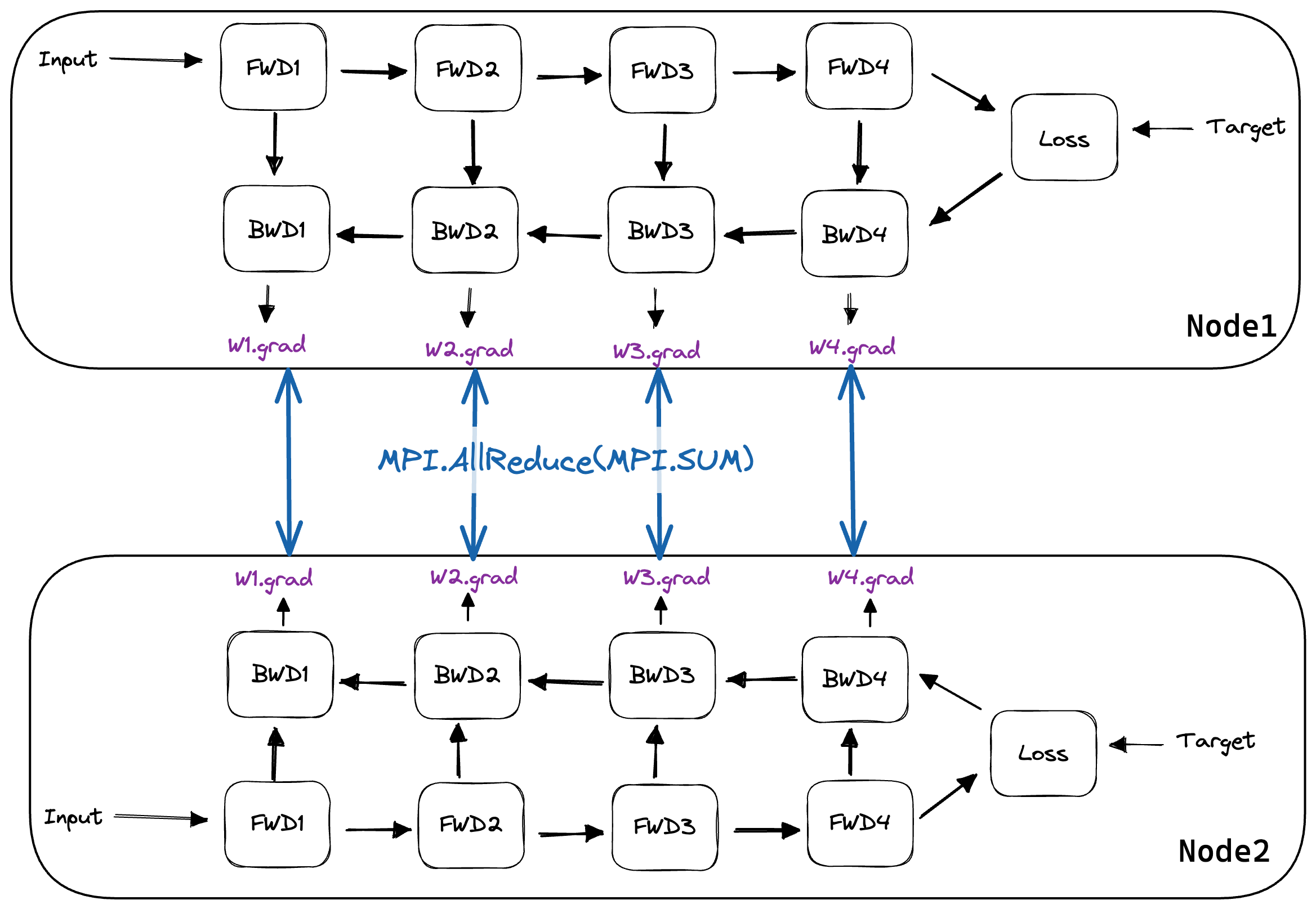
The AllReduce operation ensures that every GPU calculates the exact same average gradient, leading to an identical weight update across all model replicas. This keeps the models synchronized at every training step.

The following video segment walks through this process in the context of PyTorch's DistributedDataParallel (DDP).

A Concrete Example

Let's trace the flow with a simple numerical example, similar to the one in the video.

Imagine a trivial model $y=w\cdot x$ with a single weight $w$, which we initialize to $w=5$. We are training on two GPUs.

• GPU 0 gets data $x_0=2$.
• GPU 1 gets data $x_1=4$.

The gradient of the loss with respect to $w$ is simply $x$.

1. Forward/Backward Pass (Local Computation):

   • GPU 0 computes its local gradient: $\nabla w_0=x_0=2$.
   • GPU 1 computes its local gradient: $\nabla w_1=x_1=4$.

2. Gradient Synchronization (AllReduce):

   • An AllReduce operation is called with the local gradients as input and SUM as the reduction operation.
   • The operation calculates the global sum: $\nabla w_{global\_sum}=\nabla w_0+\nabla w_1=2+4=6$.
   • This result, 6, is distributed to both GPUs.

3. Weight Update (Local Computation):

   • Each GPU now computes the average gradient: $\nabla w_{avg}=\frac{6}{2}=3$.
   • Both GPUs perform an identical weight update using this averaged gradient (e.g., $w_{new}=w_{old}-\eta \cdot \nabla w_{avg}$).

Because both GPUs arrive at the same average gradient of 3, their model weights remain perfectly synchronized for the next iteration.

The Mechanics: How is AllReduce Implemented?

Now that we understand what AllReduce does and why it's necessary, let's briefly look at how it's implemented. A naive implementation would be a two-step process: a Reduce to a single GPU (the "root"), followed by a Broadcast from that root. This is inefficient as it creates a communication hotspot at the root GPU.

High-performance libraries like NCCL use more sophisticated, decentralized algorithms. One of the most common is the Ring-AllReduce algorithm.

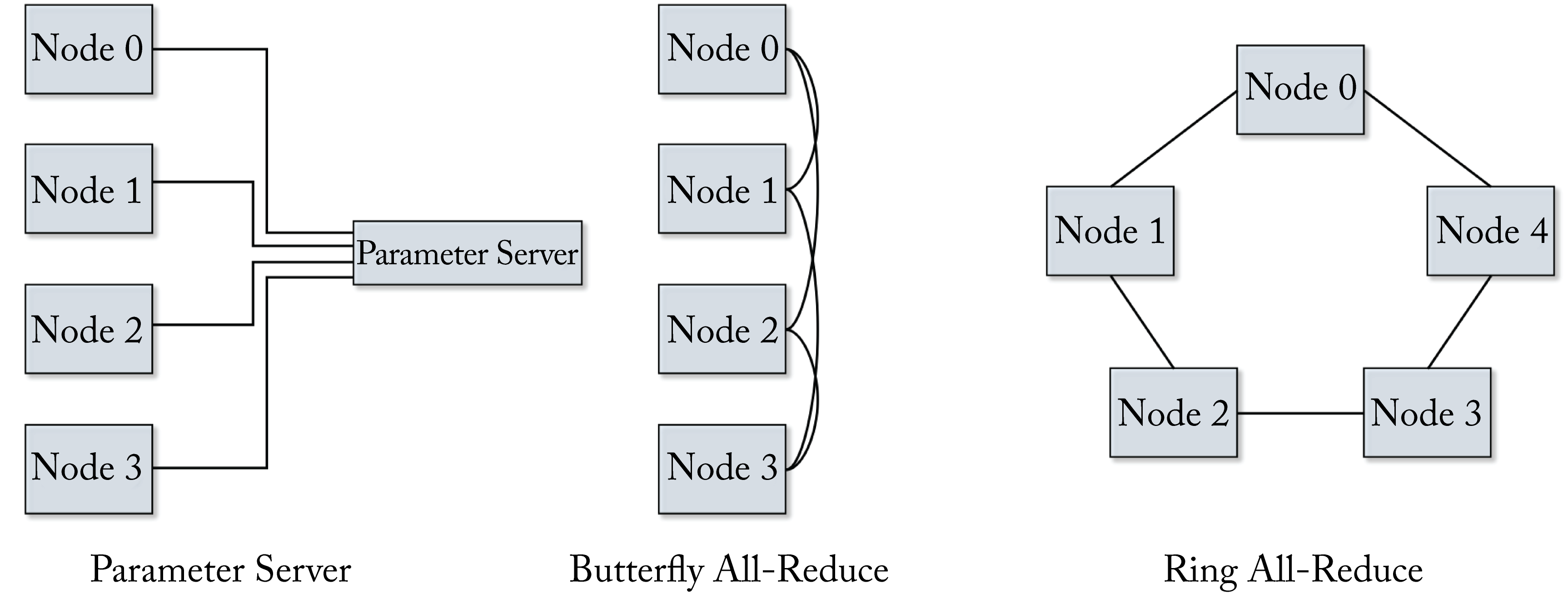
The Ring-AllReduce algorithm cleverly avoids a central bottleneck by organizing the GPUs in a logical ring. The operation proceeds in two phases: a Reduce-Scatter phase followed by an All-Gather phase.

1. Reduce-Scatter: The data on each GPU is chunked. In a series of steps, each GPU sends a chunk to its neighbor, receives a chunk from its other neighbor, and reduces the received chunk with its local data. After $N-1$ steps (for $N$ GPUs), each GPU holds a different, fully-reduced chunk of the final result.
2. All-Gather: In another series of $N-1$ steps, the GPUs circulate these reduced chunks around the ring. After this phase, every GPU has received every chunk, allowing it to reconstruct the full, final result vector.

This animation from the HOTI symposium talk on NCCL provides an excellent visualization of this process.

By structuring communication this way, the Ring algorithm can effectively saturate the communication bandwidth of all links in the ring simultaneously, making it highly efficient for large data transfers, such as the gradients of a large neural network.

Optimization: Overlapping Communication and Computation

A final, critical point for system design is that the AllReduce operation does not have to wait for the entire backward pass to finish. Modern frameworks like PyTorch DDP are more clever. As soon as the gradients for the final layers of a model are computed, the framework can begin the AllReduce operation for those gradients. This communication can then happen in parallel with the ongoing computation of gradients for the earlier layers of the model. This pipelining technique, known as communication-computation overlap, is crucial for hiding communication latency and maximizing GPU utilization.

This concept is explained in more detail in the following video, using a profiler trace to visualize the overlap.

Conclusion

In this lesson, we dissected the AllReduce collective, the workhorse of data-parallel training. You now understand its role as the essential synchronization primitive that ensures model consistency in a distributed environment.

Key Takeaways:

• Definition: AllReduce is a collective operation that performs a reduction (e.g., SUM) on input data from all GPUs and delivers the final, identical result back to all of them.
• Function in Data-Parallel Training: Its primary function is to average the locally computed gradients from all model replicas. This ensures that every GPU performs the same weight update, keeping the models synchronized throughout training.
• Mechanics: Efficient implementations like Ring-AllReduce avoid centralized bottlenecks by passing data in a logical ring, proceeding in two phases: Reduce-Scatter and All-Gather.
• System Optimization: Modern training frameworks overlap AllReduce communication with the backward pass computation to hide communication latency and improve hardware utilization.

Preview of the Next Lesson:

We have established the what and why of AllReduce and briefly touched on the how with the Ring algorithm. In our next lesson, we will perform a deeper architectural analysis of the main AllReduce algorithms. We will analyze the Ring-AllReduce and Tree-based algorithms in terms of their bandwidth usage, latency, and message size sensitivity, giving you the tools to reason about which algorithm is best suited for different hardware topologies and workload characteristics.