DCF Valuation for Real Estate in Python

Hello! Welcome to the final lesson of the "Advanced Property Valuation Techniques" module.

In the last few lessons, you've mastered the theoretical underpinnings of the most sophisticated valuation methods. You learned how to assemble a multi-year cash flow statement, calculate a property's value using the Discounted Cash Flow (DCF) method, and finally, how to reconcile that value with figures from the sales comparison and cost approaches.

Today, we bring all that theory to life. As a software engineer, you'll appreciate this transition from concept to execution. Our learning outcome is to write Python code to perform a DCF valuation for an income-producing property. We will build a functional, reusable model that translates the logic of a DCF analysis into code, culminating the work we've done throughout this module.

1. The Anatomy of a DCF Model

Before we write any code, let's revisit the structure of a typical DCF analysis. Often, these are built in spreadsheets. The image below shows a detailed 7-year DCF for a commercial property.

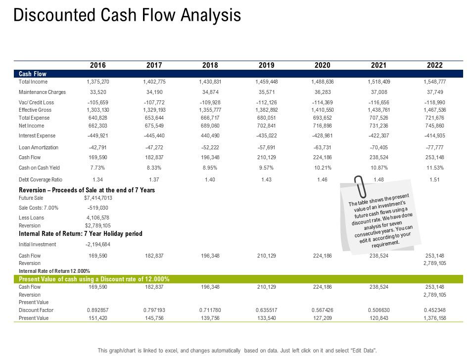
Our goal is to create a Python script that accomplishes the same thing. Our model will need to perform these key steps:

1. Define Inputs: Set our assumptions for the holding period, growth rates, vacancy, etc.
2. Project Operating Cash Flows: Build a year-by-year pro forma to calculate the Net Operating Income (NOI) and subtract Capital Expenditures (CapEx) to find the Unlevered Free Cash Flow (UFCF).
3. Calculate Reversion Value: Estimate the property's sale price at the end of the holding period.
4. Combine Cash Flows: Create a single timeline of cash flows, combining the annual UFCF with the reversion value in the final year.
5. Discount to Present Value: Apply the discount rate to bring all future cash flows back to their value today.
6. Sum for Final Value: Add up the present values to determine the property's intrinsic value based on the DCF analysis.

2. A Structured Approach to Modeling Cash Flows in Python

While you could implement this from scratch using pandas or even basic Python lists, doing so can become cumbersome and error-prone. For this lesson, we'll use a library called rangekeeper, which is specifically designed for modeling financial flows over time. Its object-oriented structure provides a robust and readable way to build our DCF, which aligns well with professional software development practices.

The following resource provides a complete walkthrough of building a DCF model using this library. We will adapt its methodology for our purpose.

3. Building the DCF Model Step-by-Step

Let's now write the code. We'll create a function that takes our key assumptions as inputs and returns the DCF value.

First, you'll need to install the necessary libraries if you haven't already:
pip install rangekeeper pandas

3.1. Defining Inputs and Setup

We start by defining all our assumptions. These will be the arguments to our main function. For the operating expenses, remember that in a real-world Spanish context, you would break this down into specific deductible items.

Here is the complete Python function. We will break down what each part does below.

import pandas as pd
import rangekeeper as rk
import locale

def calculate_dcf_value(
    initial_pgi: float,
    holding_period_years: int,
    pgi_growth_rate: float,
    opex_as_percent_of_pgi: float,
    vacancy_rate: float,
    capex_as_percent_of_pgi: float,
    exit_cap_rate: float,
    discount_rate: float
) -> float:
    """
    Performs a Discounted Cash Flow (DCF) valuation for an income-producing property.

    Args:
        initial_pgi (float): Potential Gross Income in Year 1.
        holding_period_years (int): The number of years the property is held.
        pgi_growth_rate (float): Annual growth rate for PGI.
        opex_as_percent_of_pgi (float): Operating Expenses as a percentage of PGI.
        vacancy_rate (float): Vacancy and credit loss as a percentage of PGI.
        capex_as_percent_of_pgi (float): Capital Expenditures as a percentage of PGI.
        exit_cap_rate (float): The capitalization rate used to estimate the sale price.
        discount_rate (float): The rate used to discount future cash flows.

    Returns:
        float: The calculated DCF value of the property.
    """
    # 1. SETUP: Define currency and time span for the analysis
    # Using EUR for our Spanish context.
    try:
        locale.setlocale(locale.LC_ALL, 'es_ES.UTF-8')
    except locale.Error:
        locale.setlocale(locale.LC_ALL, 'en_US.UTF-8') # Fallback for different OS setups
        
    units = rk.measure.Index.registry
    currency = rk.measure.register_currency(registry=units, currency_code='EUR')

    start_date = pd.Timestamp.now()
    analysis_span = rk.duration.Span.from_duration(
        name='Holding Period',
        date=start_date,
        duration=rk.duration.Type.YEAR,
        amount=holding_period_years
    )
    analysis_sequence = analysis_span.to_sequence(frequency=rk.duration.Type.YEAR)

    # 2. PROJECT OPERATING CASH FLOWS (PRO FORMA)
    # Potential Gross Income (PGI)
    pgi_projection = rk.projection.Extrapolation(
        form=rk.extrapolation.Compounding(rate=pgi_growth_rate),
        sequence=analysis_sequence
    )
    potential_gross_income = rk.flux.Flow.from_projection(
        name='Potential Gross Income',
        value=initial_pgi * currency.units,
        proj=pgi_projection
    )

    # Vacancy Allowance
    vacancy = rk.flux.Flow(
        name='Vacancy Allowance',
        movements=potential_gross_income.movements * -vacancy_rate
    )

    # Effective Gross Income (EGI)
    effective_gross_income = rk.flux.Stream(
        name='Effective Gross Income',
        flows=[potential_gross_income, vacancy]
    ).sum()

    # Operating Expenses (OpEx)
    operating_expenses = rk.flux.Flow(
        name='Operating Expenses',
        movements=potential_gross_income.movements * opex_as_percent_of_pgi
    ).negate()

    # Net Operating Income (NOI)
    net_operating_income = rk.flux.Stream(
        name='Net Operating Income',
        flows=[effective_gross_income, operating_expenses]
    ).sum()

    # Capital Expenditures (CapEx)
    capital_expenditures = rk.flux.Flow(
        name='Capital Expenditures',
        movements=potential_gross_income.movements * capex_as_percent_of_pgi
    ).negate()
    
    # Unlevered Free Cash Flow (UFCF)
    unlevered_free_cash_flow = rk.flux.Stream(
        name='Unlevered Free Cash Flow',
        flows=[net_operating_income, capital_expenditures]
    ).sum()

    # 3. CALCULATE REVERSION VALUE
    # First, project NOI for Year N+1
    noi_year_n = net_operating_income.movements.values[-1]
    noi_year_n_plus_1 = noi_year_n * (1 + pgi_growth_rate) # Assuming OpEx grows at same rate
    
    reversion_value_amount = noi_year_n_plus_1 / exit_cap_rate

    # Create a flow for the reversion value that occurs at the end of the holding period
    reversion_span = rk.duration.Span(
        start_date=analysis_span.end_date - pd.DateOffset(days=1),
        end_date=analysis_span.end_date
    )
    reversion_flow = rk.flux.Flow.from_projection(
        name='Reversion Value',
        value=reversion_value_amount * currency.units,
        proj=rk.projection.Distribution(
            form=rk.distribution.Uniform(),
            sequence=reversion_span.to_sequence(frequency=rk.duration.Type.YEAR)
        )
    )

    # 4. COMBINE CASH FLOWS
    total_cash_flow = rk.flux.Stream(
        name='Total Cash Flow',
        flows=[unlevered_free_cash_flow, reversion_flow],
        frequency=rk.duration.Type.YEAR
    ).sum()

    # 5. & 6. DISCOUNT AND SUM FOR FINAL VALUE
    present_values = total_cash_flow.pv(
        rate=discount_rate,
        frequency=rk.duration.Type.YEAR
    )
    
    dcf_final_value = present_values.collapse().movements.item().magnitude
    
    return dcf_final_value

# --- Example Usage ---
assumptions = {
    "initial_pgi": 60000,           # €60,000 / year
    "holding_period_years": 10,
    "pgi_growth_rate": 0.03,        # 3% per year
    "opex_as_percent_of_pgi": 0.35, # 35%
    "vacancy_rate": 0.05,           # 5%
    "capex_as_percent_of_pgi": 0.05,# 5%
    "exit_cap_rate": 0.05,          # 5%
    "discount_rate": 0.08           # 8%
}

property_value = calculate_dcf_value(**assumptions)

print(f"DCF Valuation of the property: €{property_value:,.2f}")
# Expected output might be around €675,348.16, depending on exact date calculations

Code Breakdown:

• Step 1 (Setup): We define the currency (EUR) and the time period (holding_period_years) for our analysis. rangekeeper uses Span to define time intervals.
• Step 2 (Pro Forma): This is the core of the projection.
  • potential_gross_income is created as a Flow that starts at initial_pgi and grows using a Compounding extrapolation.
  • vacancy, operating_expenses, and capital_expenditures are calculated as simple percentages of PGI. Note the use of .negate() for outflows.
  • We use Stream to combine flows. effective_gross_income is a stream of PGI and Vacancy, which we then .sum() into a single resultant flow. This process is repeated to get to unlevered_free_cash_flow.
• Step 3 (Reversion Value): We calculate the NOI for the year after our holding period (noi_year_n_plus_1), divide it by the exit_cap_rate to get the future sale price, and create a reversion_flow that occurs only in the last year.
• Step 4 (Combine): We create a final Stream that adds the annual unlevered_free_cash_flow and the reversion_flow.
• Step 5 & 6 (Discount & Sum): The .pv() method neatly calculates the present value of each cash flow in our total stream using the discount_rate. Then, .collapse().movements.item().magnitude sums up these present values into a single number, our final DCF valuation.

Conclusion

Congratulations on completing the "Advanced Property Valuation Techniques" module! You've successfully translated the complex theory of Discounted Cash Flow analysis into a functional and reusable Python model. This is a powerful skill that combines your financial knowledge with your software engineering expertise.

Key Takeaways:

• A DCF valuation model can be systematically built in Python by projecting operating cash flows and the reversion value, and then discounting them to the present.
• Libraries like rangekeeper provide helpful abstractions (Flow, Stream, Span) that enforce a structured, object-oriented approach to financial modeling.
• The output of a DCF model is highly sensitive to its input assumptions, particularly the discount rate and the exit cap rate.
• The code provides a template that can be expanded to include more detailed, country-specific line items, such as the Spanish deductible expenses we noted.

Preview of the Next Module:
We now pivot from valuation (what is an asset worth?) to performance measurement (how good is an investment in that asset?). In our next module, "Advanced Performance and Risk-Adjusted Returns," we will start by exploring a fundamental metric that every investor cares about: the equity multiple. You will learn to calculate this metric to understand the total cash return on your invested equity over the lifetime of a project.