Comparative Market Analysis: Valuing Properties

Hello! Welcome back to our module on advanced property valuation.

In our last lesson, we outlined the methodology of the Sales Comparison Approach (SCA), the cornerstone of property valuation. We discussed the principle of substitution, the importance of finding good comparables or "testigos," and the Spanish method of "homogeneización" using coefficients.

Today, we move from theory to practice. Your learning outcome is to select appropriate comparable properties and apply adjustments to determine a property's value. We will walk through a complete, step-by-step example, starting with a list of potential comparables and ending with a final value estimate. This structured, rule-based process is something you'll likely find very familiar, as it closely mirrors an algorithmic approach to problem-solving.

1. The Subject Property and the Search for Comparables

Let's begin with our subject property. We want to determine its market value. The data is adapted from a real Spanish valuation case.

Subject Property Data:

• Type: Apartment in a multi-story building
• Location: Bajamar, La Laguna (Tenerife)
• Constructed Area: 58.29 m²
• Bedrooms: 2
• Bathrooms: 1
• Age: Built in 1968 (Let's assume the valuation year is 2023, making it 55 years old)
• Condition: Normal
• Construction Quality: Medium
• Floor: 2nd floor

Our first task is to search the market (e.g., on portals like Idealista, Fotocasa) for recently sold properties that are as similar as possible. After a search, we have a list of six potential comparables.

When selecting the best comparables from a list, you'd filter based on:

1. Recency: All these sales are recent, which is good. Spanish regulations for official appraisals require data from the last 6 months.
2. Proximity: All are in the same general area (Bajamar). We will still account for micro-location differences.
3. Similarity: All are apartments. However, they differ in size, age, condition, and quality. These are the differences we will need to adjust for.

For this exercise, we'll assume all six are suitable enough to be included in our analysis, as is common in a formal appraisal to ensure a robust data set.

2. The Adjustment Grid and Homogenization Coefficients

Now for the core of the analysis: adjusting the sale prices of the comparables to make them equivalent to our subject property. We organize this work in an adjustment grid.

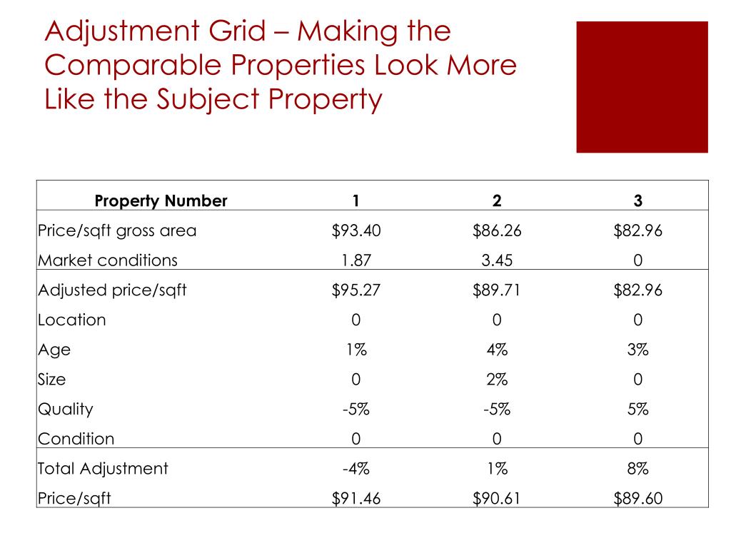
The guiding principle remains:

• If the comparable is superior to the subject, we adjust its price downwards (coefficient < 1).
• If the comparable is inferior to the subject, we adjust its price upwards (coefficient > 1).

To understand this logic intuitively, let's watch a short video.

Applying Adjustments: A Detailed Walkthrough of Comparable 1

Let's apply this to Comparable 1 from "Tabla 8" of the document you reviewed.

• Comparable 1: Sells for €105,000 (€1,750/m²). It has 1 bedroom, Baja quality, Bueno conservation, was built in 2017 (6 years old), and is on the ground floor.
• Subject: 2 bedrooms, Media quality, Normal conservation, built in 1968 (55 years old), on the 2nd floor.

We need to compare them feature by feature. The specific coefficient values often come from an appraiser's internal database and experience, but we can use the guide values provided in the reference document.

Here is the step-by-step adjustment for Comparable 1:

1. Location (Ubicación): The appraiser deemed them "Similar," but with a slight disadvantage for the comp, warranting a minor downward adjustment. In the final example in LINK, a coefficient of 0.990 is used. This implies the subject's location is slightly better.
2. Building Quality (Cali Edific): Comp is "Baja," Subject is "Media." The comp is inferior. To make it equivalent to the subject, we must adjust its price up. We apply a majorador (increasing) coefficient. The example uses 1.075.
3. Condition (Conservación): Comp is "Bueno" (Good), Subject is "Normal." The comp is superior. We must adjust its price down. We apply a minorador (decreasing) coefficient. The example uses 0.980.
4. Age (Antigüedad): Comp is from 2017 (6 years), Subject is from 1968 (55 years). The comp is much newer and therefore superior. We must adjust its price down significantly. The example uses 0.755. Logic: A large part of its €1,750/m² price is due to its newness. If it were 55 years old like our subject, it would have sold for much less.
5. Floor (Planta): Comp is ground floor, Subject is 2nd floor. In many markets, higher floors are more desirable (more light, less noise). Let's assume the 2nd floor is superior. We adjust the comp's price down. The example uses 0.980.
6. Layout/Bedrooms (Programa): Comp has 1 bedroom, Subject has 2. The comp is inferior. We must adjust its price up. The example in LINK calls them "Coincidente" but applies a coefficient of 0.990. This is a bit counter-intuitive; a more logical approach would be a coefficient > 1. This highlights that official appraisals can have nuances, but for our purpose, let's follow the example's value.
7. Surface Area (Superficie): Comp is 60m², Subject is 58.29m². They are very similar. The example uses a coefficient of 1.024. According to "Tabla 4," larger properties sometimes have a lower price per square meter, so a smaller property (our subject) would command a higher €/m² value, hence the upward adjustment for the comp.

3. Calculating the Homogenized Value

We now have a set of coefficients for Comparable 1. How do we combine them? While the UPV video suggested multiplying them, a common method in Spanish appraisals, and the one used in our reference document, is to calculate a single resultant coefficient.

The formula provided in LINK is:
$\text{Coef resultante}=1+(\sum \text{Coeficientes}-n)$
where n is the number of parameters adjusted.

However, the practical example in the document seems to use a simpler multiplicative approach to arrive at the final Coef Result. Let's re-calculate to confirm:
0.990 * 1.075 * 0.980 * 0.755 * 0.980 * 0.990 * 1.024 = 0.786. The table shows 0.79. This confirms they are multiplying the coefficients. This is the more direct method.

• Resultant Coefficient for Comp 1: 0.79
• Comparable 1 Unit Price: €1,750/m²
• Homogenized Unit Value (VH): €1,750/m² * 0.79 = €1,389.40/m²

This adjusted value is our estimate of what Comparable 1 would have sold for, on a per-square-meter basis, if it had the same characteristics as our subject property.

We repeat this process for all six comparables.

4. Reconciliation and Final Value Estimate

After the homogenization process, we have a range of adjusted unit values:

• Comp 1: €1,389.40/m²
• Comp 2: €2,102.34/m²
• Comp 3: €2,441.58/m²
• Comp 4: €2,013.47/m²
• Comp 5: €1,866.78/m²
• Comp 6: €2,132.37/m²

The final step is to reconcile these into a single value. A simple arithmetic mean is one option.

Arithmetic Mean:
$\frac{1389.40+2102.34+2441.58+2013.47+1866.78+2132.37}{6}=\text{€1,990.99/m²}$

A more sophisticated approach is a weighted average, where you give more weight to the comparables that are most similar to the subject (i.e., those whose resultant coefficient is closest to 1.0). In our case, Comparable 2 (Coef: 1.02) and Comparable 4 (Coef: 0.87) are the most similar and would receive higher weights. For simplicity, we will stick with the arithmetic mean used in the example.

Final Market Value Calculation:
$\text{Value}=\text{Homogenized Unit Value}\times \text{Subject Area}$
$\text{Value}=1,990.99€/m^2\times 58.29m^2=\text{€116,054.80}$

Our final estimate for the market value of the subject property is approximately €116,000.

Test your understanding!

Suppose you find a new comparable, Comp 7. It sold for €2,500/m². It is identical to your subject property in all aspects except that it has a brand new, luxury kitchen (your subject has a standard, older kitchen).

1. Is Comp 7 superior or inferior to your subject property?
2. Should the adjustment coefficient for the kitchen be greater or less than 1?
3. Will the homogenized unit value for Comp 7 be higher or lower than €2,500/m²?

Show answer

1. Superior. The luxury kitchen makes it better than the subject property.
2. Less than 1. Because the comparable is superior, you must adjust its price downwards. You would use a minorador coefficient (e.g., 0.95).
3. Lower. The adjustment will reduce the comp's unit price to reflect what it would have sold for without the luxury kitchen, bringing it in line with the subject.

From Manual Analysis to Code

As a software engineer, you can see that this entire process is a structured algorithm:

1. Input: Subject property features, database of comparable sales.
2. Filter: Select comparables based on proximity, date, and type rules.
3. Loop: For each selected comparable:
   • Compare each feature (feature_i) to the subject's feature.
   • Apply a rule-based function get_coefficient(comp_feature, subject_feature) to find the adjustment coefficient.
   • Multiply all coefficients to get a resultant coefficient.
   • Calculate the homogenized value.
4. Aggregate: Calculate a weighted average of all homogenized values.
5. Output: Final estimated property value.

This is a classic problem for a Case-Based Reasoning (CBR) system. The following resource is a simple Python project that does exactly this.

Conclusion

Today you have moved beyond the theory of the Sales Comparison Approach and learned how to apply it. You now know how to select relevant comparables and, most importantly, how to execute the systematic process of "homogeneización" by applying adjustment coefficients to account for differences in property characteristics. This allows you to arrive at a data-driven, defensible estimate of a property's market value.

Key Takeaways:

• The SCA starts with selecting the most similar, recent, and proximate comparables ("testigos").
• An adjustment grid is used to systematically compare the subject and comps feature by feature.
• For each feature, if a comp is superior, its value is adjusted down (coef < 1); if it's inferior, its value is adjusted up (coef > 1).
• The individual coefficients are combined (often multiplicatively) into a single resultant coefficient for each comp.
• The final value is determined by taking a reconciled average (simple or weighted) of the comps' homogenized unit values and multiplying by the subject's area.
• This entire process is algorithmic and can be modeled programmatically.

Preview of the Next Lesson:
While the SCA is the most common valuation method, it's not the only one. What if you're valuing a unique property with no recent comparables, like a church or a school? In our next lesson, we will explore an alternative method by learning to explain the cost approach and when it is applicable for valuation.