Estimating Carbon Emissions from Land-Use Change: Methods and Uncertainties

Hello! Welcome back.

In our last lesson, we performed a 'back-of-the-envelope' calculation for global CO₂ emissions from fossil fuel combustion. We found that a simple model based on energy consumption data could produce an estimate (~10 GtC/yr) remarkably close to official figures. This gave us a solid understanding of how the largest source of anthropogenic carbon is quantified.

Introduction

Today, we turn our attention to the second major source of anthropogenic emissions: Land-Use Change (LUC). While smaller in magnitude than fossil fuels (typically estimated at 1-2 GtC/yr), its contribution is significant, and the process of estimating it is fraught with challenges and uncertainties.

This lesson will delve into the methodologies used to quantify these emissions. You'll find that the problem combines elements of large-scale data analysis, remote sensing, and complex systems modeling. Given your background in statistical science and economics, you will appreciate the parallels with econometric modeling, where different approaches (e.g., bottom-up accounting vs. top-down process models) are used to understand a complex system with incomplete information.

By the end of this lesson, you will be able to: Describe the methodologies and uncertainties involved in estimating carbon emissions from land-use change.

1. The Scale and Challenge of Land-Use Change Emissions

Land-use change refers to the human alteration of land cover, which releases or absorbs carbon. The primary driver is deforestation, the conversion of forests to agricultural land (cropland or pasture). Other significant activities include forest degradation (e.g., selective logging), the drainage of carbon-rich peatlands, and changes in farming practices.

When a forest is cleared, the carbon stored in trees, plants, and soil is released into the atmosphere, primarily as CO₂. This happens rapidly if the biomass is burned, and more slowly if it's left to decay.

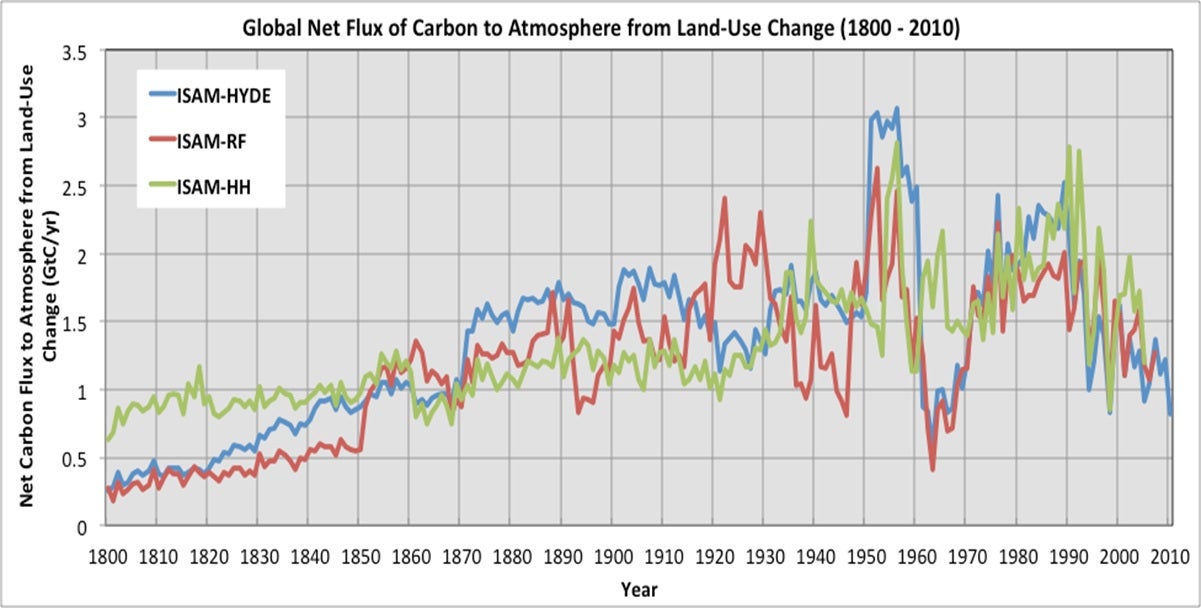
The image below shows historical estimates of this carbon flux. Notice the two key features: the general upward trend, especially since 1900, and the divergence between the different estimation models. This immediately highlights the core theme of today's lesson: uncertainty.

To place these emissions in context, the next image compares various estimates of LUC emissions with those from fossil fuels.

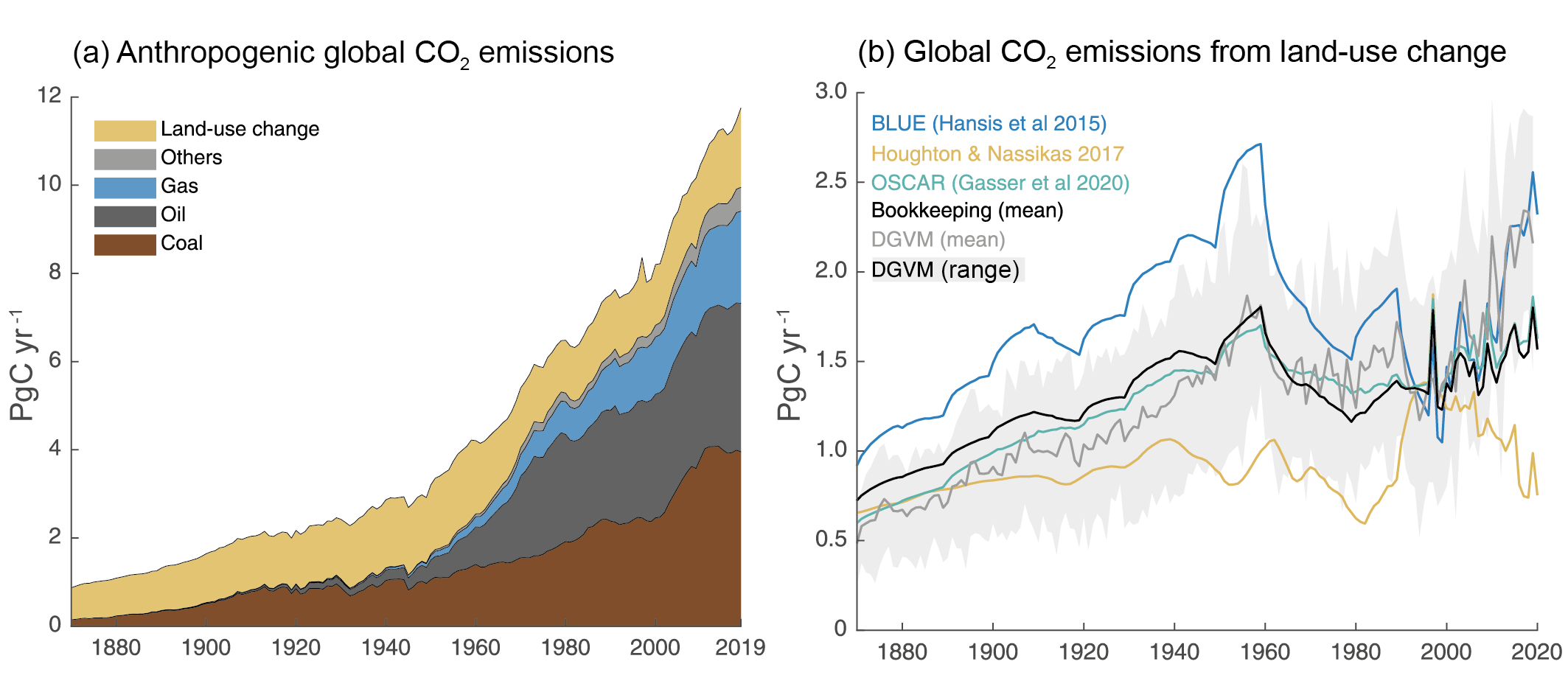
Graph (b) introduces the two main families of methodologies we will discuss: Bookkeeping models and Dynamic Global Vegetation Models (DGVMs).

2. Methodologies for Estimating LUC Emissions

Estimating LUC emissions is fundamentally a two-part problem:

1. How much land area has changed from one type to another (e.g., forest to cropland)?
2. What is the change in carbon stock associated with that conversion?

The two primary methods tackle this problem from different perspectives.

As the IPCC report highlights, the two main approaches are:

A. Bookkeeping Models (Bottom-Up)

This approach is analogous to the accounting method we used for fossil fuels. It "keeps the books" on carbon stocks as land is converted.

• Method: It starts with data on land-use changes, often from national statistics (like the FAO) or satellite imagery. It then multiplies the area of converted land by an emission factor, which is the difference in carbon density between the original and new land cover.
  $\text{Emissions}={\sum }_{\text{transitions}}\text{Area Changed}\times ({\text{Carbon Density}}_{\text{initial}}-{\text{Carbon Density}}_{\text{final}})$
• Data: Requires historical land-use data and spatially explicit maps of carbon stocks in vegetation and soils.
• Strengths: Conceptually straightforward and transparent. The results can be directly traced back to the input data on land area and carbon density.
• Weaknesses: These models are largely diagnostic. They don't typically capture dynamic feedback processes, such as the effect of higher CO₂ levels or a changing climate on plant growth (the so-called "non-anthropogenic sink" mentioned in the IPCC text).

B. Dynamic Global Vegetation Models (DGVMs) (Process-Based)

DGVMs are complex simulations of the Earth's land surface.

• Method: Instead of just accounting, DGVMs model the underlying physical and biological processes: photosynthesis, respiration, decomposition, and competition between plant types. They are driven by climate data and atmospheric CO₂ concentrations, and human land-use change is applied as an external forcing.
• Data: Requires climate inputs (temperature, precipitation), atmospheric CO₂ data, soil maps, and land-use change scenarios.
• Strengths: Can simulate the interaction between ecosystems and the climate system, including feedbacks. They can be used for future projections under different climate and land-use scenarios.
• Weaknesses: They are computationally intensive and their complexity can make them opaque. The results are sensitive to the parameterization of many biophysical processes, making them difficult to validate.

The discrepancy mentioned in the IPCC report (0.1 ± 1.0 GtCO₂ yr⁻¹ from inventories vs. 5.1 ± 2.6 GtCO₂ yr⁻¹ from bookkeeping models) arises partly from differences in definitions (e.g., what constitutes "managed forest") and partly from what processes are included.

3. A Deeper Dive: Indirect Land-Use Change (iLUC)

One of the most complex and debated areas of LUC accounting is indirect land-use change (iLUC). This occurs when a policy or activity causes land-use change in another location through market mechanisms.

The classic example is biofuels. If the U.S. decides to grow more corn for ethanol on existing agricultural land, that land is no longer available to grow corn for food. This reduces the global food supply, driving up prices. In response, farmers elsewhere—say, in Brazil—may convert a forest or savanna into new cropland to capitalize on the higher prices. The emissions from that deforestation in Brazil are an indirect consequence of the U.S. biofuel policy.

Modeling iLUC requires coupling economic models with biophysical models. This is a perfect illustration of the interdisciplinary nature of climate science, blending economics, statistics, and Earth system science.

The following resource from the California Air Resources Board (ARB) provides an excellent, in-depth look at how this is done in practice for regulatory purposes. It is a technical document, but it clearly lays out the methodology.

The ARB report illustrates a state-of-the-art methodology:

1. An economic shock (e.g., increased demand for biofuel) is introduced into a global economic model (GTAP-BIO).
2. The model calculates a new economic equilibrium, which includes changes in land use around the world as farmers respond to price signals.
3. The output—hectares of land converted from one type to another (e.g., forest to cropland) in specific regions—is fed into a separate biophysical model (the AEZ-EF model).
4. The AEZ-EF model uses detailed emission factors to calculate the resulting GHG emissions from changes in above-ground biomass, soil carbon, etc.

This multi-model chain is a powerful tool, but as we will now see, it is also a major source of uncertainty.

4. Sources of Uncertainty

Uncertainty is the defining characteristic of LUC emission estimates. It stems from every step of the process, from data collection to modeling choices.

A. Data Uncertainty

• Land Cover Change: Satellite data can be ambiguous. Is a patch of forest lost due to clear-cutting for agriculture, a forest fire, or selective logging? Definitions of "forest" or "degradation" vary between studies and countries.
• Carbon Stocks: The amount of carbon in a forest or soil is highly variable. A single "emission factor" for "tropical forest" masks immense diversity. Measuring soil carbon, especially at depth, is difficult and expensive. The ARB report's AEZ-EF model (Attachment 2, Part 7) goes into great detail on the components they model—deadwood, litter, understory biomass, harvested wood products—each with its own data sources and uncertainties.

B. Model Uncertainty

• Structural Choices: The choice between a bookkeeping model and a DGVM is a primary source of difference. As we saw, they can produce very different results due to what processes they include.
• Parameter Uncertainty: This is a critical issue, especially in the economic models used for iLUC. The results are highly sensitive to assumptions about economic parameters.
  • Yield Price Elasticity (YPE): The ARB report has an entire appendix (Attachment 1, Part 6) dedicated to this single parameter. It determines how much crop yields increase in response to higher prices. A high elasticity means farmers can produce more on existing land, reducing the need to clear new land and thus lowering iLUC emissions. As the attachment shows, economists have a wide range of estimates for this value, leading to significant uncertainty in the model output.
  • Land Transformation Elasticity (ETL): This governs how easily land can be converted from one use to another (e.g., pasture to cropland). This is another key parameter with high uncertainty.
• Time Accounting: A large pulse of CO₂ is emitted when a forest is cleared. How should this one-time emission be allocated to the fuel produced from that land over many years? The ARB report discusses this in Attachment 3 (Part 8). A 30-year amortization period (used by ARB and the EPA) yields a higher annual emission value than a 100-year period. This is a subjective methodological choice, not a scientific fact.

C. Quantifying Uncertainty

Given these many sources of uncertainty, how do scientists put bounds on their estimates? The ARB report provides a clear answer.

As you read, the use of Monte Carlo Simulation (MCS) is a powerful technique to propagate uncertainty through the complex model chain. By defining probability distributions for key input parameters (like YPE, carbon stocks, etc.), running the model thousands of times, and analyzing the distribution of the outputs, they can characterize the uncertainty in the final iLUC value. This is a standard and robust approach in statistical modeling and risk analysis.

Conclusion

Today we've explored the complex and uncertain world of estimating carbon emissions from land-use change. Unlike the relatively straightforward accounting for fossil fuels, quantifying LUC emissions requires grappling with incomplete data, competing modeling philosophies, and deep-seated parameter uncertainty.

Key Takeaways:

• Emissions from Land-Use Change (LUC) are a significant component of the global carbon budget, primarily driven by deforestation for agriculture.
• The two main estimation methodologies are bookkeeping models (bottom-up, accounting-based) and Dynamic Global Vegetation Models (DGVMs) (process-based simulations).
• Indirect Land-Use Change (iLUC), often driven by biofuel policies, is a major challenge that requires linking global economic models (like GTAP) with biophysical emissions models.
• Uncertainties are large and stem from every part of the process:
  • Data: Inconsistent and incomplete data on both land-cover change and carbon stocks.
  • Models: Structural differences between models and high sensitivity to key parameters, particularly economic elasticities in iLUC models.
  • Methodology: Subjective choices, such as the time horizon for amortizing emissions, significantly impact the final numbers.

In this and the previous lesson, we have quantified the two primary sources of anthropogenic carbon. But where does it all go? In our next lesson, we will analyze the partitioning of anthropogenic CO₂ emissions between the atmosphere, ocean, and land biosphere sinks, which ultimately determines the rate of climate change.