Global Carbon Budget: CO2 Partitioning

Hello! Welcome to your next lesson.

Introduction

In our last two lessons, we quantified the two primary sources of anthropogenic carbon emissions: fossil fuel combustion (~10 GtC/yr) and land-use change (~1-2 GtC/yr). We established that these are the inputs disturbing the Earth's natural carbon cycle.

The crucial question now is: where does all this emitted CO₂ go? The answer determines the rate at which CO₂ accumulates in the atmosphere and, consequently, the pace of climate change.

Today, we will analyze the partitioning of anthropogenic CO₂ emissions. We will investigate how these emissions are distributed among the three major reservoirs that act as "sinks": the atmosphere, the oceans, and the land biosphere. Our primary tool for this analysis will be the Global Carbon Budget, an annual synthesis of data from research groups around the world.

This process is analogous to a large-scale accounting or econometric exercise. We have measured inputs (emissions) and we need to track them as they flow into different stocks (sinks). You'll see that, just like in complex economic models, the books don't perfectly balance, leaving a "residual" or "imbalance" term that reflects the limits of our measurement and understanding.

By the end of this lesson, you will be able to: Analyze the partitioning of anthropogenic CO₂ emissions between the atmosphere, ocean, and land biosphere sinks, using data from the Global Carbon Budget.

1. The Global Carbon Budget: An Accounting Framework

The Global Carbon Budget is a massive annual effort by the Global Carbon Project to collate data and establish a consistent picture of the carbon cycle. The fundamental principle is one of conservation of mass, which we can express as a simple budget equation:

Total Emissions = Total Sinks

This can be broken down into its five core components:

Where:

• $E_{FOS}$ = Emissions from Fossil Fuels and industry (e.g., cement production).
• $E_{LUC}$ = Net emissions from Land-Use Change.
• $G_{ATM}$ = Growth in atmospheric CO₂ concentration (the portion that remains in the atmosphere).
• $S_{OCEAN}$ = The net uptake of CO₂ by the ocean sink.
• $S_{LAND}$ = The net uptake of CO₂ by the terrestrial (land) sink.
• $B_{IM}$ = The Budget Imbalance, a term that captures the discrepancy between the independently estimated sources and sinks. A small imbalance indicates that our understanding and measurements are largely consistent.

The diagram below, from a recent Global Carbon Budget report, provides a clear visual summary of this partitioning.

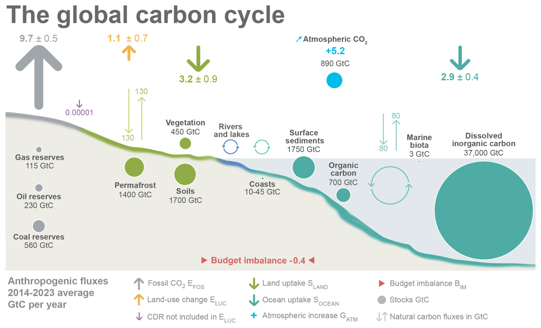
Take a moment to study this diagram. You can see the two sources we've studied, $E_{FOS}$ (9.7 GtC/yr) and $E_{LUC}$ (1.1 GtC/yr), for a total emission of 10.8 GtC/yr. This is then partitioned into the three sinks: land uptake (3.2 GtC/yr), ocean uptake (2.9 GtC/yr), and the residual atmospheric increase (5.2 GtC/yr). Note the small budget imbalance of -0.4 GtC.

2. Analyzing the Partitioning with the Global Carbon Budget Report

To understand how these numbers are derived and how they've changed over time, we will dive into a detailed walkthrough of the Global Carbon Budget 2023 report.

After watching the video, let's perform the budget calculation for 2022 using the figures provided (from Part 1 of the video):

• Sources:

  • $E_{FOS}$ = 9.9 GtC/yr
  • $E_{LUC}$ = 1.2 GtC/yr
  • Total Emissions = 11.1 GtC/yr

• Sinks:

  • $G_{ATM}$ = 4.6 GtC/yr
  • $S_{OCEAN}$ = 2.8 GtC/yr
  • $S_{LAND}$ = 3.8 GtC/yr
  • Total Sink Uptake = 11.2 GtC/yr

• Imbalance:

  • $B_{IM}=(\text{Total Emissions})-(\text{Total Sink Uptake})$
  • $B_{IM}=11.1-11.2=-0.1$ GtC/yr

As the video presenter notes, this very small imbalance gives us confidence that the scientific community has a robust and consistent understanding of the major carbon flows.

3. A Closer Look at the Sinks

Now let's analyze the proportion of emissions that goes into each sink. Using the 2022 data:

• Atmosphere: $\frac{4.6}{11.1}\approx 41\%$
• Ocean: $\frac{2.8}{11.1}\approx 25\%$
• Land: $\frac{3.8}{11.1}\approx 34\%$

These percentages are relatively stable over recent decades. Let's examine each sink in more detail.

The Airborne Fraction

The portion of CO₂ that remains in the atmosphere is arguably the most important single number in climate science. It is formally known as the airborne fraction.

Airborne Fraction = (Annual increase in atmospheric CO₂) / (Total annual emissions)

For 2022, this was about 41%. Looking at decadal averages, this value has remained surprisingly constant at around 45-48% for the last 60 years, even as emissions have quadrupled. This implies that the ocean and land sinks have scaled their uptake in proportion to our emissions—a fortunate but not guaranteed state of affairs.

The diagram in the 2021 report shows:

• Total Emissions (2011-2020 avg): 34.8 (Fossil) + 4.1 (LUC) = 38.9 GtCO₂/yr
• Atmospheric Growth: 18.6 GtCO₂/yr (48%)
• Ocean Sink: 10.2 GtCO₂/yr (26%)
• Land Sink: 11.2 GtCO₂/yr (29%)

(Note: These figures are in GtCO₂. To convert to GtC, divide by ~3.664. The percentages remain the same.)

The Ocean and Land Sinks

The ocean and land sinks each absorb roughly a quarter to a third of our emissions.

• Ocean Sink: CO₂ dissolves from the atmosphere into the surface ocean. This process is governed by the difference in partial pressure of CO₂ between the air and the sea. As shown in the Beckwith video (Part 5, not assigned but you can review from 22:35), colder waters (like the North Atlantic and Southern Ocean) are strong sinks, while warmer tropical waters can be sources.
• Land Sink: This is primarily driven by photosynthesis. The increase in atmospheric CO₂ can directly stimulate plant growth, a phenomenon known as CO₂ fertilization. The land sink is much more variable year-to-year than the ocean sink, largely due to climate variations like the El Niño-Southern Oscillation (ENSO), which can cause widespread droughts and fires, temporarily weakening the sink.

A critical area of research is whether these sinks will continue to keep pace with emissions. As the planet warms, these sink processes can be compromised.

This feedback mechanism—where warming weakens the very sinks that are mitigating it—is a major source of concern and a key topic in climate modeling, which we will touch on in a future module.

Conclusion

In this lesson, we have moved from quantifying the sources of anthropogenic CO₂ to tracking where it goes. By analyzing the Global Carbon Budget, we've established a clear accounting framework for the partitioning of emissions.

Key Takeaways:

• Anthropogenic CO₂ emissions are partitioned into three main sinks: the atmosphere, the oceans, and the land biosphere.
• The Global Carbon Budget provides a comprehensive accounting framework: $E_{FOS}+E_{LUC}=G_{ATM}+S_{OCEAN}+S_{LAND}+B_{IM}$.
• For the last decade, the approximate partitioning has been:
  • ~48% remains in the atmosphere (the "airborne fraction").
  • ~26% is absorbed by the ocean.
  • ~29% is absorbed by the land biosphere.
• The small budget imbalance term reflects the high consistency of independent measurements and gives us confidence in our understanding of the overall cycle.
• The land and ocean sinks have so far scaled with emissions, but their future efficiency is a critical uncertainty as climate change may weaken their capacity to absorb CO₂.

We now have a clear picture of how much CO₂ we emit and what fraction of it stays in the atmosphere each year. However, this doesn't tell us how long that CO₂ persists. In our next and final lesson of this module, we will model the decay of an atmospheric CO₂ pulse using a multi-box model to understand its long residence time.