Transform Arrays with NumPy Indexing, Broadcasting, and Vectorization

Hello! In the previous lesson, you separated reusable calculations from the script that runs them. Now you can make those calculations work on whole collections of numbers without writing a Python loop for every element.

This lesson focuses on three NumPy tools: indexing to select data, broadcasting to combine arrays of compatible shapes, and vectorization to express a numerical transformation over an entire array. These are everyday tools for preparing machine-learning features and calculating prediction errors. Allow about 40 minutes, including the short videos and time to run the examples.

---

Select the numbers you need

In your project’s isolated environment, install NumPy if it is not already available:

python -m pip install numpy

Update the project’s dependency record after installing it. In the examples below, np is the conventional short name for NumPy.

import numpy as np

features = np.array([
    [2., 4.],
    [4., 6.],
    [6., 8.],
    [8., 10.]
])

print(features.shape)  # (4, 2)

Think of features as four observations, each with two numerical features. Its shape tells you there are four rows and two columns. NumPy indices start at zero: features[1, 0] is 4.0, the value in the second row and first column.

Watch the indexing demonstrations in numpy tutorial - slicing/stacking arrays, indexing with boolean arrays by codebasics:

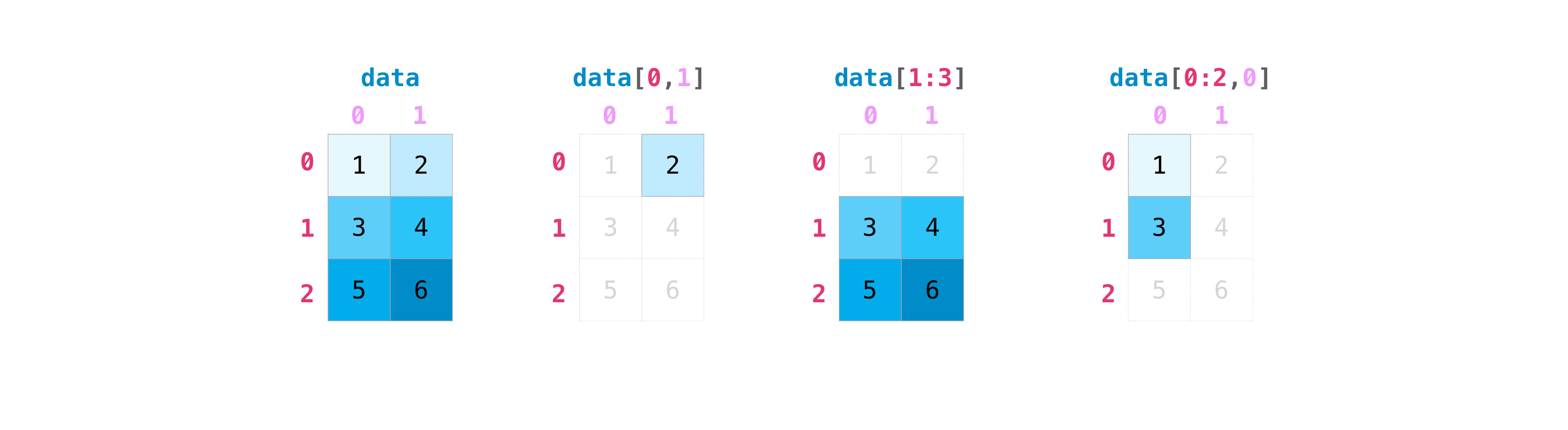
For our features array, an integer index selects one position along an axis; a slice selects a range. The stop of a slice is excluded:

print(features[1, 0])     # 4.0
print(features[1:3])       # rows 1 and 2; shape (2, 2)
print(features[:, 0])      # first column of every row; shape (4,)
print(features[1:3, 0])   # first-column values from rows 1 and 2

Notice the shape distinction: features[:, 0] has shape (4,), not (4, 1). An integer index removes that axis; a slice such as features[:, 0:1] retains it. Check .shape whenever a selection will feed another calculation.

---

Filter rows—and know when you have a view

A comparison across an array produces an array of True and False values. You can use that Boolean mask as an index. Watch the later portion of the same codebasics video:

Suppose you want observations whose first feature is at least 4:

eligible = features[:, 0] >= 4
print(eligible)           # [False  True  True  True]

selected = features[eligible]
print(selected.shape)     # (3, 2)
print(selected)
# [[ 4.  6.]
#  [ 6.  8.]
#  [ 8. 10.]]

The mask has one entry per row, so indexing with it keeps complete rows. In contrast, features[features >= 6] applies a condition to individual cells and returns the matching values in a one-dimensional array. Choose the mask to match what you mean to select.

You can also request rows by their integer positions, including positions that are not adjacent:

chosen = features[[0, 2]]
print(chosen.shape)       # (2, 2)

There is a practical difference between that selection and a slice. A basic slice usually gives a view of the original data; Boolean and integer-array indexing give copies. Watch the focused explanation in Advanced NumPy Course - Vectorization, Masking, Broadcasting & More by NeuralNine:

You can see the difference without changing our features example:

original = np.array([1., 2., 3.])
view = original[:2]
view[0] = 99.
print(original)           # [99.  2.  3.]

independent = original[[0, 1]]
independent[0] = 0.
print(original)           # still [99.  2.  3.]

If you need an independent array from a slice, use .copy(). Being explicit about this is especially valuable when one transformation should not silently change the data used by another.

---

Let shapes do the repetition

Often you need the same operation for every observation. Suppose the two features have different offsets. Instead of looping over rows, you can add a two-element array:

offsets = np.array([1., 2.])
adjusted = features + offsets

print(adjusted)
# [[ 3.  6.]
#  [ 5.  8.]
#  [ 7. 10.]
#  [ 9. 12.]]

This works by broadcasting. NumPy aligns shapes from their rightmost dimensions. For each aligned pair, the sizes must be equal, or one must be 1; a missing leading dimension is treated like 1. Here (4, 2) and (2,) are compatible: the two offsets are applied across all four rows.

Watch NeuralNine’s explanation of the shape rules:

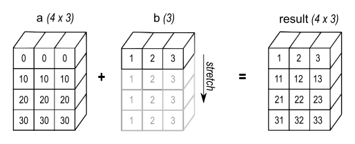
Shape checks can also prevent mistakes. A (4,) array cannot be added to our (4, 2) features: comparing from the right gives 4 and 2, which are incompatible. If four numbers are intended as one adjustment per row, give them a column axis:

row_adjustments = np.array([0., 1., 2., 3.])
print(row_adjustments[:, np.newaxis].shape)  # (4, 1)

by_row = features + row_adjustments[:, np.newaxis]
print(by_row.shape)                          # (4, 2)

np.newaxis inserts a dimension of length one. Here each row’s adjustment is applied to both columns. Shape is therefore more than a description of storage: it helps specify which values should combine.

---

Express the whole transformation

Vectorization means expressing array operations directly, rather than writing an explicit Python loop for each element. NumPy can then carry out those element-wise operations using its array machinery. For example, the prediction-error function from the previous lesson built errors one pair at a time. With arrays, the subtraction and absolute value operate on all pairs:

actual = np.array([2., 4., 6.])
predicted = np.array([1., 5., 5.])

errors = np.abs(actual - predicted)
print(errors)             # [1. 1. 1.]
print(np.mean(errors))    # 1.0

Read the brief “Working with mathematical formulas” portion of NumPy’s absolute basics for beginners for another example involving squared prediction errors:

One caution: broadcastable prediction and target arrays are not necessarily correctly paired arrays. A target of shape (3, 1) and predictions of shape (3,) can broadcast to a (3, 3) result, comparing every target with every prediction. If your intention is three paired errors, check for identical shapes first:

def mean_absolute_error_np(actual, predicted):
    """Return the mean absolute error for equally shaped, nonempty arrays."""
    actual = np.asarray(actual, dtype=float)
    predicted = np.asarray(predicted, dtype=float)

    if actual.shape != predicted.shape or actual.size == 0:
        raise ValueError("inputs must have the same nonempty shape")

    return np.mean(np.abs(actual - predicted))

Finally, bring selection and broadcasting together in a feature transformation. Each column has its own center and scale; NumPy applies both two-element arrays across the selected rows:

center = np.array([5., 7.])
scale = np.array([2., 4.])

transformed = (selected - center) / scale
print(transformed.shape)  # (3, 2)
print(transformed)
# [[-0.5  -0.25]
#  [ 0.5   0.25]
#  [ 1.5   0.75]]

The first transformed row comes from [4., 6.]: its entries are (4 - 5) / 2 and (6 - 7) / 4. NumPy performs that same per-column calculation for every selected row. No explicit loop is needed, and the output remains a two-feature array.

---

What to take forward

Indexing chooses where a transformation applies; broadcasting determines how shapes align; vectorized operations describe what happens to all the selected values. When results look surprising, inspect .shape first, then ask whether your selection is a view or a copy.

The next lesson moves from element-wise transformations to matrix operations. There, dimensions will still matter—but matrix multiplication will follow different rules from the +, -, and / operations used here.