The Memory Wall: Scaling to Trillion-Parameter Models

Introduction

Welcome to the fifth lesson of the "Emerging Architectures and Future Trends" module. In our previous lesson, we explored how emerging standards like CXL and UCIe provide powerful tools for building composable systems, tackling resource limitations at the system and package levels. These standards are, in essence, engineering responses to a fundamental and escalating challenge in high-performance computing.

This lesson drills down into the core of that challenge. Our learning outcome is to: Analyze the memory capacity and bandwidth challenges ('the memory wall') when scaling to trillion-parameter models. We will dissect the two critical facets of this problem:

1. The Memory Capacity Wall: The sheer size of modern models vastly exceeds the memory available on any single accelerator.
2. The Memory Bandwidth Wall: The rate at which data can be supplied to compute units lags far behind the growth in computational power, leading to underutilized, "starving" processors.

By the end of this lesson, you will have a quantitative understanding of why these "walls" are the primary obstacles to scaling AI and appreciate the architectural and algorithmic context for many of the optimization techniques we have discussed throughout this course.

Part 1: The Widening Chasm Between Compute and Memory

The "memory wall" is not a new concept in computer architecture; it describes the growing disparity between the speed of processors and the speed of the memory that feeds them. However, the explosive growth of AI has pushed this problem to an extreme.

To begin, let's watch a short video that frames the memory wall in the context of modern AI hardware.

The video articulates the central issue: hardware compute capability, measured in Floating Point Operations Per Second (FLOPs), has been scaling at a much faster exponential rate than memory bandwidth.

Let's look at this trend graphically.

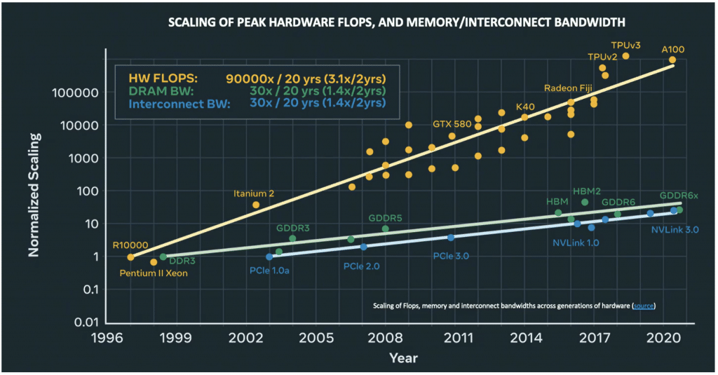
This trend is formalized in the paper "AI and Memory Wall," which we will refer to throughout this lesson.

This disparity means that for many workloads, the performance bottleneck is not how fast we can compute, but how fast we can move data to the compute units.

Part 2: The Two Faces of the Memory Wall for Trillion-Parameter Models

When scaling to models with a trillion or more parameters, the memory wall manifests as two distinct, yet interconnected, challenges: a crisis of capacity and a crisis of bandwidth.

A. The Capacity Wall: Where Do We Store the Model?

The first and most immediate problem is that the memory required to hold a large model's state during training far exceeds the capacity of a single GPU.

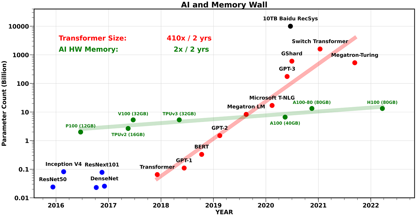
To train a model, we need to store more than just its parameters (weights). The primary components are:

1. Parameters ($\Psi$): The model's weights.
2. Gradients ($\nabla \Psi$): The same size as the parameters, computed during the backward pass.
3. Optimizer States: Data required by the optimizer to update the weights. For the common Adam optimizer, this includes momentum and variance terms, typically stored in 32-bit floating point (FP32).
4. Activations: Intermediate results from the forward pass that are saved for use in the backward pass.

Let's quantify the memory required for the model states (parameters, gradients, and optimizer states), using the Adam optimizer and mixed-precision training as a reference. The video "Ultimate Guide To Scaling ML Models" provides an excellent breakdown.

As the video explains, for a model with $\Psi$ parameters, the memory footprint is approximately:

• Parameters: $\Psi$ parameters in 16-bit precision (FP16) = $2\Psi$ bytes.
• Gradients: $\Psi$ parameters in FP16 = $2\Psi$ bytes.
• Optimizer States (Adam):
  • FP32 copy of parameters: $4\Psi$ bytes.
  • Momentum (FP32): $4\Psi$ bytes.
  • Variance (FP32): $4\Psi$ bytes.
• Total: $2\Psi +2\Psi +4\Psi +4\Psi +4\Psi =\text{16}\Psi$ bytes.

For a 1 trillion parameter model ($\Psi =10^{12}$):

An NVIDIA H100 GPU has 80 GB of High-Bandwidth Memory (HBM). To simply store the model states—without even considering activations—would require:

This calculation makes it clear that training trillion-parameter models is fundamentally a distributed systems problem. It's impossible to do on a single device. This is the primary motivation for memory-saving techniques like ZeRO (Zero Redundancy Optimizer), which partitions these states across GPUs instead of replicating them, a topic we covered in Module 8.

B. The Bandwidth Wall: Starving the Beast

Even if a model or a piece of a model fits in GPU memory, we face the second challenge: feeding the compute units fast enough to keep them busy. The key metric for understanding this is Arithmetic Intensity.

Arithmetic Intensity is the ratio of floating-point operations (FLOPs) performed to the bytes of data moved from memory (Memory Operations or MOPs).

• High Arithmetic Intensity: The workload is compute-bound. Many calculations are performed for each byte of data loaded. Matrix-matrix multiplications (GEMM) on large matrices are a classic example.
• Low Arithmetic Intensity: The workload is memory-bandwidth-bound. The processor spends most of its time waiting for data. Matrix-vector multiplications (GEMV) are a classic example.

The paper "AI and Memory Wall" provides an excellent case study comparing a BERT-style encoder model with a GPT-style decoder model.

The critical insight here is that autoregressive generation, the process of producing one token at a time in models like GPT, is dominated by matrix-vector operations. To generate a single token, the entire model's weight matrices must be streamed from HBM to the compute units, which then perform relatively few operations before the next token requires the same process. This is a workload with extremely low arithmetic intensity, making it severely bottlenecked by memory bandwidth.

The Latency Wall: An Ultimate Limit

As we scale to even larger clusters to overcome capacity and bandwidth limits, a more fundamental barrier emerges: the latency wall. This concept, explored in a recent paper by Epoch AI, posits that at a certain scale, the fixed time delay (latency) of network communication becomes the dominant factor, creating a hard ceiling on performance.

The latency wall suggests that simply adding more GPUs will eventually yield no benefit, as the time for each training step becomes limited by the speed of light and network protocol overhead, not by the number of available processors.

Part 3: Strategies for Tackling the Memory Wall

The entire field of large-scale AI systems is, in many ways, an ongoing battle against the memory wall. The solutions are a mix of algorithmic, software, and hardware innovations, many of which we've covered in previous modules.

• Algorithmic/Software Solutions:

  • Reducing Memory Footprint: Techniques like Mixed-Precision Training (using FP16/BF16) and Quantization (INT8/INT4) reduce the size of parameters and activations. Activation Checkpointing trades re-computation for memory, while ZeRO and FSDP partition model states. These directly attack the capacity wall.
  • Increasing Arithmetic Intensity: Operator Fusion combines multiple small kernels (e.g., an activation function followed by a normalization layer) into one larger kernel, reducing the number of round trips to main memory and thus increasing the FLOP-to-byte ratio.

• Hardware and System Solutions:

  • On-Chip Memory: Increasing the size and bandwidth of on-chip caches (SRAM) and on-package memory (HBM) is a continuous effort.
  • System-Level Interconnects: As we saw last lesson, CXL allows for memory expansion and tiering, providing a larger, if slower, pool of memory that can alleviate capacity pressure for certain data (like optimizer states).
  • Multi-GPU Interconnects: High-bandwidth, low-latency interconnects like NVLink/NVSwitch and InfiniBand are critical for mitigating the communication overhead forced upon us by the memory capacity wall (as we saw in Module 5).

Conclusion

This lesson has delved into the fundamental constraints that define the landscape of large-scale AI. The relentless growth in model size has collided with the physical limits of data movement, creating a two-front war against the memory wall.

Key Takeaways:

• The Memory Wall in AI is the stark and growing divergence between the scaling of compute power (FLOPs) and the scaling of memory capacity and bandwidth.
• The Capacity Wall is a direct consequence of model size. A trillion-parameter model requires terabytes of memory for its states, making distributed training on hundreds of GPUs an absolute necessity.
• The Bandwidth Wall is a function of arithmetic intensity. Many AI workloads, especially autoregressive inference, are memory-bound, meaning performance is limited by data transfer speeds, not computation.
• At extreme scales, a Latency Wall emerges, where the fundamental delay of network communication sets a hard limit on how fast training can proceed, regardless of how many GPUs are added.
• Overcoming these walls requires a holistic approach, combining algorithmic innovations (ZeRO, checkpointing), software optimizations (fusion), and advanced hardware systems (HBM, CXL, NVLink).

Preview of the Next Lesson

We have established that the memory wall forces us to distribute models across many devices, turning a single-node problem into a massive distributed systems challenge. This distribution introduces its own severe bottleneck: communication. Our next and final lesson of this module, "Analyze the interconnect and communication bottlenecks that arise when training models at extreme scale," will examine this problem in detail, exploring the performance characteristics and limitations of the interconnects that tie these large systems together.