Optimizing Logistic Regression with Gradient Descent

Hello! Welcome to the next lesson in our journey through the mathematical foundations of machine learning.

In our previous session, we accomplished a crucial task: we derived the gradient of the logistic regression cost function. We found that for the average cross-entropy loss $J(\mathbf{\theta })$, the partial derivative with respect to a single parameter ${\theta }_j$ is:

With the cost function and its gradient, we now have a map of the "error surface" and a compass that points in the direction of steepest ascent. Today's lesson is about using that compass to find the lowest point on the map. We will apply the gradient descent algorithm to iteratively find the optimal set of parameters $\mathbf{\theta }$ that minimizes our cost function, effectively training our model.

This lesson is the bridge between the pure calculus of the last session and a functional machine learning algorithm.

1. The Gradient Descent Algorithm: A Formal View

You've likely encountered gradient descent in your practical work, but your goal is to master the theory. So, let's move beyond the common analogy of "walking downhill" and formally establish why the algorithm works. The core idea is to take a small step in the direction opposite to the gradient, which is guaranteed to decrease the function's value, provided the step is small enough.

We can prove this using a Taylor approximation. For a deeper, more rigorous explanation of this process, the following resource is an excellent read.

The General Update Rule

As shown in the reading, the argument culminates in a simple, powerful, iterative update rule. Starting with an initial guess for the parameters ${\mathbf{\theta }}^{(0)}$, we repeatedly update them at each step $t$:

Let's break this down:

• ${\mathbf{\theta }}^{(t)}$ is the vector of parameters at iteration $t$.
• $\alpha$ is the learning rate, a scalar hyperparameter that controls the size of our step.
• ${\nabla }_{\mathbf{\theta }}J({\mathbf{\theta }}^{(t)})$ is the gradient of the cost function evaluated with the current parameters.

This update is performed for each parameter ${\theta }_j$ in the vector $\mathbf{\theta }$ simultaneously.

2. Gradient Descent for Logistic Regression

Now, let's make this concrete by substituting the specific gradient for logistic regression that we derived in the last lesson.

The update rule for a single parameter ${\theta }_j$ becomes:

Here, $h_{{\mathbf{\theta }}^{(t)}}({\mathbf{x}}^{(i)})=\sigma (({\mathbf{\theta }}^{(t)}{)}^T{\mathbf{x}}^{(i)})$ is the model's prediction for example $i$ using the parameters from step $t$.

The Guarantee of Convergence: Convexity

A critical question is whether this iterative process will find the best possible parameters. For many complex models, gradient descent can get stuck in "local minima"—valleys that aren't the lowest point on the entire error surface.

Fortunately, for logistic regression, this is not a concern. The cross-entropy loss function is convex. A convex function has a bowl-like shape, meaning it has only one minimum, which is the global minimum.

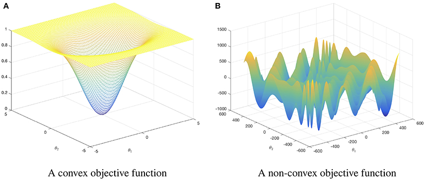
Andrew Ng also discusses this important property in his CS229 lecture.

3. A Worked Example

Let's trace one single step of gradient descent to make this tangible. The following resource provides a clear walkthrough.

Let's recap the example from the text.

• Input: $\mathbf{x}=[x_1,x_2{]}^T=[3,2{]}^T$, with true label $y=1$.
• Initial Parameters: $w_1=0,w_2=0,b=0$. (Using $w,b$ notation here, equivalent to $\theta$).
• Learning Rate: $\eta =0.1$.

1. Calculate Prediction ($\hat{y}$ or $h$):
   The linear part is $z=\mathbf{w}\cdot \mathbf{x}+b=(0)(3)+(0)(2)+0=0$.
   The prediction is $\hat{y}=\sigma (z)=\sigma (0)=\frac{1}{1+e^0}=0.5$.

2. Calculate Gradient: The gradient of the loss for this single example w.r.t each parameter is $(\hat{y}-y)x_j$.

   • $\frac{\partial L}{\partial w_1}=(\hat{y}-y)x_1=(0.5-1)(3)=-1.5$
   • $\frac{\partial L}{\partial w_2}=(\hat{y}-y)x_2=(0.5-1)(2)=-1.0$
   • $\frac{\partial L}{\partial b}=(\hat{y}-y)=(0.5-1)=-0.5$
     So, $\nabla L=[-1.5,-1.0,-0.5{]}^T$.

3. Update Parameters: ${\mathbf{\theta }}^{(1)}={\mathbf{\theta }}^{(0)}-\eta \nabla L$.

   • $w_1^{(1)}=0-(0.1)(-1.5)=0.15$
   • $w_2^{(1)}=0-(0.1)(-1.0)=0.10$
   • $b^{(1)}=0-(0.1)(-0.5)=0.05$

After just one step, the weights have been nudged in a direction that will make the prediction for this example closer to the true label. This process is repeated until the parameters converge.

4. Practical Aspects of Gradient Descent

The update rule we've used so far, which sums over all $n$ training examples for every single update, is known as Batch Gradient Descent. In practice, there are variations with different trade-offs.

The Learning Rate

The learning rate $\alpha$ is arguably the most important hyperparameter.

• If $\alpha$ is too small: Convergence will be very slow, requiring many iterations.
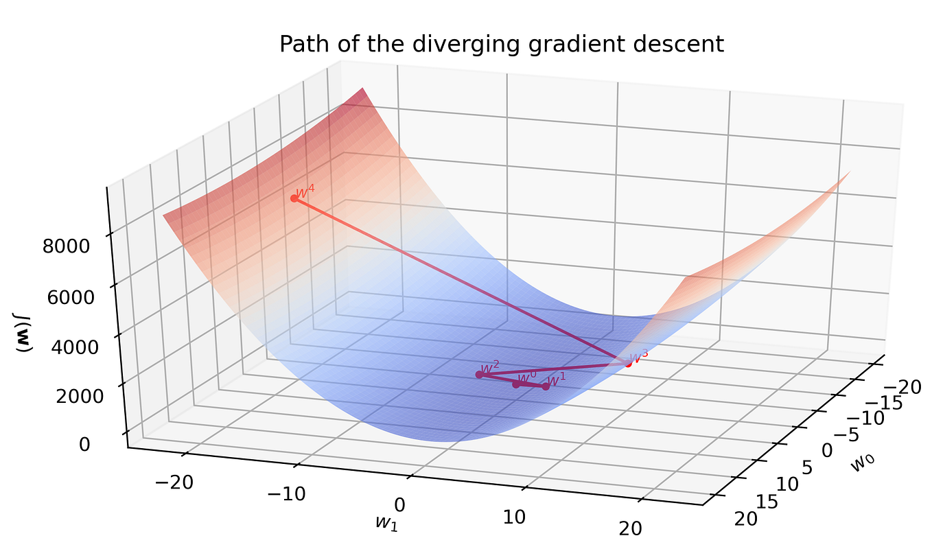
• If $\alpha$ is too large: The algorithm can "overshoot" the minimum and fail to converge. The cost might oscillate or even diverge (increase) with each step.

Batch, Stochastic, and Mini-Batch Gradient Descent

The choice of how many examples to use for computing the gradient in each update step leads to three main variants. The Jurafsky and Martin text provides an excellent summary.

Here is a summary:

1. Batch Gradient Descent:

   • Update: Uses the entire training set ($n$ examples) to compute the gradient for one parameter update.
   • Pros: Stable, straight path towards the minimum.
   • Cons: Very computationally expensive and slow on large datasets.

2. Stochastic Gradient Descent (SGD):

   • Update: Uses a single training example to compute the gradient and update the parameters.
   • Pros: Much faster updates. Allows for online learning.
   • Cons: The path to the minimum is very noisy ("stochastic"). The cost function may fluctuate heavily.

3. Mini-Batch Gradient Descent:

   • Update: Uses a small batch of examples (e.g., 32, 64, 128) to compute the gradient.
   • Pros: A compromise that offers the best of both worlds. It's computationally efficient due to vectorization and provides a more stable convergence than SGD.
   • Cons: Introduces another hyperparameter: the batch size.

In modern deep learning and machine learning, mini-batch gradient descent is the most common approach.

Conclusion

In this lesson, we put the gradient to work. We formally defined the gradient descent algorithm and proved why it is guaranteed to reduce our cost function. By combining this algorithm with the specific gradient for logistic regression, we now have a complete recipe for training the model.

Key Takeaways:

• The gradient descent update rule is ${\mathbf{\theta }}^{(t+1)}:={\mathbf{\theta }}^{(t)}-\alpha {\nabla }_{\mathbf{\theta }}J({\mathbf{\theta }}^{(t)})$.
• We can prove that this update reduces the cost function using a Taylor series approximation.
• Because the cross-entropy loss for logistic regression is a convex function, gradient descent is guaranteed to find the unique global minimum.
• The learning rate ($\alpha$) is a critical hyperparameter that balances convergence speed and stability.
• Mini-Batch Gradient Descent is the most common optimization strategy in practice, offering a balance between computational efficiency and update stability.

Preview of the Next Lesson:
We have now covered how to define, derive, and optimize a logistic regression model to find the best parameters $\mathbf{\theta }$. But what do these learned parameters actually represent? In our next lesson, we will explore the geometric interpretation of $\mathbf{\theta }$ and see how it defines the decision boundary that the model uses to separate the classes.