Production Data Workload Requirements: Throughput, Latency, Scalability, and Availability

Welcome. This course begins with the operational language used to reason about production data systems. Before tuning Spark, choosing partitions, or diagnosing shuffles, you need to be able to state what the workload must achieve—and recognize when two apparently similar requirements are actually different.

In this lesson, you will distinguish throughput, latency, scalability, and availability for data workloads, then turn vague expectations such as “near real time” or “highly scalable” into measurable requirements. The focus is on pipelines and data-serving systems rather than any one tool.

---

Four different questions about one workload

Consider a pipeline that ingests product events, enriches them, and makes them available to dashboards.

The four concepts answer distinct questions:

Property	Core question	Typical units	Example requirement
Throughput	How much work can the system complete over time?	events/s, rows/min, GB/hour	Sustain 80,000 events/s
Latency	How long does one unit of work take?	ms, s, min	99% of events available within 5 minutes
Scalability	Can capacity grow with demand while requirements remain met?	capacity under a defined growth test	At 3 times peak load, maintain the stated SLOs after adding workers
Availability	When asked to perform its function, is the service usable?	percentage of eligible requests or time	99.95% of valid ingestion requests are accepted and durably recorded

The terms are related, but they are not interchangeable.

• A system can process a very large volume every hour while individual records wait a long time before processing.
• A system can respond quickly to a small load but fail when traffic rises.
• A system can be fast when it is working, yet unavailable during a dependency outage.
• A system can have many servers and still fail to scale if a single overloaded partition or database key limits the whole workload.

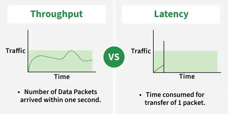
Throughput: completed work per unit time

For data engineering, throughput should name both the unit of work and the boundary at which it is measured. “The pipeline handles 10,000 per second” is incomplete. Does that mean:

• 10,000 events accepted by the ingestion API per second?
• 10,000 events parsed and validated per second?
• 10,000 records written to the lakehouse per second?
• 10,000 records made queryable by downstream users per second?

These can differ substantially. A Kafka producer may accept events quickly while consumer lag grows, so input throughput looks healthy even though useful output throughput is insufficient.

A useful capacity distinction is:

• Arrival rate: how fast new work enters the system.
• Completion rate: how fast the system finishes that work.
• Backlog: work that has arrived but is not yet complete.

If the sustained completion rate is below the arrival rate, backlog grows. Eventually, records become late, queues fill, retry traffic rises, and the system may start rejecting work. Thus, a throughput requirement is usually about the maximum sustained completion rate, not a brief benchmark peak.

Latency: elapsed time for one item of work

Latency measures duration for an individual request, event, or job. For data workloads, first establish the clock’s start and finish:

• Request latency: from an API request arriving to a response being returned.
• Ingestion latency: from an event being produced to its durable acceptance.
• Processing latency: from a record becoming available to a processor until transformation completes.
• End-to-end freshness latency: from event creation to correct data becoming visible in the final destination.

For a business-facing pipeline, end-to-end latency is usually the one that matters. A daily report can be computed quickly once the scheduled job begins, but if it starts six hours after data arrives, the stakeholder experiences six-hour freshness latency.

Latency should almost never be specified only as an average. A mean can look healthy while a meaningful minority of records is severely delayed. Production targets therefore commonly use percentiles:

• p50 describes the median experience.
• p95 is the value at or below which 95% of observations fall.
• p99 exposes the slow tail that affects one in every hundred requests or events.

A target such as “average processing time below 30 seconds” can hide a pipeline where 95% of events complete in 2 seconds and 5% wait 10 minutes. A more operational target is: “99% of valid events are available in the serving table within 5 minutes.”

---

Availability is usability, not speed

Availability asks whether a system can successfully provide its intended function for eligible work. It does not ask how quickly it does so.

For a serving API, an availability indicator often takes this form:

$$\text{Availability}=\frac{\text{successful eligible requests}}{\text{all eligible requests}}$$

For an event-ingestion service, a “successful” request might mean that a valid event was accepted and durably persisted. For a dashboard, it might mean that a query returns a correct, current-enough result. The definition needs to exclude requests that are malformed or outside the supported contract; otherwise client bugs can distort the operational measure.

Availability targets are often written in “nines.” Their practical implications can be surprisingly different. For a continuously expected service over a 30-day month:

$$\text{Allowed downtime}=(1-\text{availability target})\times \text{time period}$$

Target	Approximate allowed downtime per 30-day month
99%	7 hours 12 minutes
99.9%	43 minutes
99.99%	4 minutes 19 seconds

The numbers are not a universal promise: planned maintenance policy, partial degradation, and the definition of a successful request all matter. But they show why a requirement for an extra nine has major architectural and operational consequences.

For a batch pipeline, availability may not be the primary user-facing requirement. A finance pipeline that runs nightly can tolerate the scheduler being briefly unreachable at 2 a.m. if it still completes before the reporting deadline. Its more meaningful objective might be job completion and data freshness. Conversely, an ingestion endpoint that feeds fraud decisions may need both high availability and very low latency.

A key operational lesson: errors and slowness can converge under overload. Queueing causes latency to rise first; timeouts and rejected requests then often reduce measured availability. Monitoring the properties separately helps identify whether the immediate problem is capacity, a failed dependency, or both.

---

Scalability: preserving behavior as demand changes

Scalability is not “having autoscaling enabled,” and it is not merely a count of machines. It is the ability of a system to accommodate a specified change in load or data size while continuing to meet the relevant throughput, latency, and availability objectives.

A scalable pipeline must be evaluated against a concrete growth shape:

• Volume: more events, records, bytes, files, or partitions.
• Rate: a higher sustained arrival rate or sharper bursts.
• Cardinality: more distinct users, keys, or groups.
• Skew: more activity concentrated on a small subset of keys.
• Concurrency: more independent queries, jobs, or consumers.
• Data history: more retained partitions and larger tables.

This specificity matters. A Spark pipeline may scale well as input files become larger, yet not scale for a group-by aggregation when one customer account produces half the records. Adding workers cannot fully solve work concentrated in one partition. Similarly, an autoscaling policy may eventually provide enough workers but react too slowly to a short, intense traffic spike.

A defensible scalability requirement includes the expected load and the performance that must survive it. For example:

At three times the current peak event rate, with the projected distribution of customer IDs, the pipeline automatically reaches sufficient worker capacity within 10 minutes and continues to process 99% of valid events end-to-end within 5 minutes.

This is testable. “The pipeline is horizontally scalable” is an architectural hope, not a requirement.

---

Turning expectations into measurable SLOs

An SLI is the measurement. An SLO is the target applied to that measurement. The operational discipline is to define both before selecting a technology or tuning a job.

Suppose a team operates a clickstream pipeline used by product dashboards and alerting. A weak requirement might be:

Process events at scale in near real time with high availability.

A production-ready version separates the concerns:

Concern	SLI definition	Example SLO
Input throughput	Valid events durably accepted per second	Sustain 100,000 events/s for four hours; handle 250,000 events/s for 10-minute bursts
End-to-end latency	Time from producer timestamp to data becoming queryable	99% within 5 minutes; 99.9% within 15 minutes
Availability	Fraction of valid ingestion requests durably accepted	At least 99.95% per calendar month
Scalability	SLO compliance under forecast growth test	At 3 times peak rate, add capacity automatically and retain the three targets above
Correctness	Fraction of sampled or reconciled events represented accurately	At least 99.99% of validated events match the source contract

Correctness is included because speed without trustworthy output has little value in data engineering. It is not one of this lesson’s four performance and reliability concepts, but it constrains their interpretation. For example, acknowledging an event before it is safely recorded may improve apparent request latency and availability while making the real pipeline less reliable.

The following short video reinforces the distinction between individual completion time and aggregate rate, including the role of latency percentiles.

Define the population and the clock

Many misleading SLOs fail because the unit and boundaries are underspecified. Before publishing one, make four choices explicit:

1. Population: Which requests or records count? For example, valid events only, excluding malformed payloads.
2. Start time: Does the clock begin when the producer creates the event, when the broker accepts it, or when Spark reads it?
3. Completion condition: Is work “done” after durable storage, transformation, table commit, or query visibility?
4. Measurement window: Is the target measured per minute, daily, weekly, or monthly? A monthly availability target can hide a severe short outage; a one-minute throughput average can hide a damaging ten-second burst.

This prevents a familiar failure mode: every individual team reports that its stage is healthy, but the end-to-end dataset is late. Per-stage telemetry remains essential for diagnosis, but end-to-end objectives represent the customer’s outcome.

---

The trade-offs you should expect

These properties pull on one another. The correct response is not to optimize every metric independently, but to decide what the workload needs most.

Throughput and latency

Batching is a classic example. Larger batches can use network, disk, and compute resources more efficiently, often raising throughput. Yet an event must wait for a batch to fill or for the next scheduled run, adding latency. A nightly ETL job may sensibly optimize throughput and cost; a fraud-event pipeline may prioritize freshness instead.

Concurrency can increase throughput until a resource saturates. Beyond that point, additional concurrent work competes for CPU, disk, memory, network, locks, or remote-service capacity. Latency rises due to waiting, and throughput may flatten or even decline.

Scalability and workload distribution

Horizontal scaling works best when work is divisible and evenly distributed. It is less effective when the bottleneck is centralized:

• a single database writer,
• one hot partition key,
• one heavily contended table or object,
• shared metadata services,
• a fixed network or storage limit.

Therefore, a capacity test needs representative key distribution, file sizes, query patterns, and concurrency. Testing only uniformly distributed synthetic data can produce a confident but false scalability claim.

Availability and latency

Availability mechanisms often introduce trade-offs. Extra replicas and automatic failover can keep service available when individual machines fail. However, coordination, health checks, cross-region communication, and stronger write confirmation may add latency. The appropriate choice depends on what a failure means for the workload. A billing event and an advertising impression can reasonably have different objectives.

---

A requirement card for a production workload

Before implementation or tuning, a compact requirement card can guide design discussions:

Field	Example
Customer outcome	Product events are visible in operational dashboards
Work unit	One valid product event
Arrival pattern	100,000 events/s sustained; 250,000 events/s campaign bursts
Throughput objective	Completion rate keeps pace with sustained arrival rate
Latency objective	99% queryable within 5 minutes; 99.9% within 15 minutes
Availability objective	99.95% of eligible ingestion requests accepted and durable monthly
Scalability test	Meet objectives at 3 times current peak and projected key skew
Measurement location	Producer timestamp through serving-table visibility
Degradation policy	Preserve priority business events; delay low-priority enrichment if constrained
Correctness guardrail	Reconcile sampled output against source events

The card does not dictate whether to use Spark, Flink, Kafka, a warehouse, or a particular database. It makes the eventual technology choice accountable to observable behavior.

---

Key takeaways

• Throughput is the amount of completed work per unit time; name the work unit and measurement boundary.
• Latency is elapsed time for one request or record, ideally measured end to end and reported with percentiles.
• Availability is the fraction of eligible work for which the service is usable and successful; it is separate from speed.
• Scalability is the ability to preserve required behavior as a specified load characteristic grows. Autoscaling can support it, but does not demonstrate it on its own.
• Production requirements become useful when they define the population, timing boundaries, percentile or rate, measurement window, and workload conditions.

Next, the course moves from requirements to architecture: you will select a data-partitioning strategy based on access patterns and workload distribution.