Selecting Data-Partitioning Strategies for Access Patterns and Workloads

Welcome back. In the previous lesson, you separated requirements such as throughput, latency, scalability, and availability. Partitioning is one of the main architectural tools for meeting those requirements as data volume and request rates grow—but it only helps when the partition layout reflects how data is actually read, written, and distributed.

This lesson develops a practical selection method. You will distinguish the partition key from the strategy that places keys onto partitions, compare hash, range, lookup, list, and geographic approaches, and make a defensible choice for common data workloads.

---

Partitioning is both grouping and routing

A partitioned dataset is still logically one table, topic, or collection, but its records are stored in smaller physical units. In a distributed database, these units are often called shards. In an analytical lake, they may be directory partitions or separate files grouped by a partition value. The terminology changes, but the architectural question is the same:

Which records should live together, and how does the system find them?

Two decisions are often mistakenly collapsed into one.

1. Choose a partition key. This determines which records are grouped together. Examples include tenant_id, customer_id, event_date, or region.
2. Choose a placement strategy. This determines which physical partition receives a particular key value: a hash function, a value range, a lookup directory, or a geographic rule.

For a simple hash layout, the placement rule might be:

$$\text{partition}=h(\text{key})\mathrm{mod}N$$

where $h$ is a hash function and $N$ is the number of partitions. The formula is deterministic: the same key is routed to the same partition.

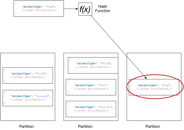
The primary benefit is not merely that each machine holds fewer rows. A good layout lets the system direct most important requests to one relevant partition rather than searching every partition. That reduces I/O, network fan-out, coordination, and tail latency.

A poor layout creates the opposite condition:

• one partition receives most writes;
• a popular key overloads a single node;
• a time-range scan must touch every partition;
• a simple query requires cross-partition joins or aggregation;
• adding capacity requires an expensive data migration.

The partition key is therefore an operational design decision, not just a schema field.

---

Start with the workload, not the data model

A key may look natural in a schema and still be wrong for the workload. Selecting a partitioning strategy starts by describing the work, using the requirement language from the previous lesson.

For each major operation, identify:

• Access predicate: What does a request specify? A tenant_id? A date interval? A region? An order ID?
• Access shape: Is it a point lookup, a range scan, an aggregation, a join, or a bulk deletion?
• Read and write distribution: Which values receive the most requests, writes, or bytes?
• Co-location requirement: Which records are commonly read or updated together?
• Growth pattern: Will new data arrive in order of time, by tenant, by region, or unpredictably?
• Lifecycle needs: Must data be deleted, archived, or moved in predictable batches?
• Boundary constraints: Are there regional latency or data-residency requirements?

A partition key is strong when it satisfies three core properties:

Property	Meaning	Why it matters
High cardinality	It has many possible values.	The system has enough groups to distribute across many partitions.
Even effective distribution	Data volume and request load are reasonably spread across values.	One partition is less likely to become a bottleneck.
Query alignment	Frequently used queries include the key.	Requests can be routed to a small number of partitions, ideally one.

Two important qualifications prevent superficial choices.

First, high cardinality is necessary but not sufficient. user_id may have millions of values, but one celebrity account can still receive more traffic than all other accounts combined. The data might be evenly distributed while the requests are not.

Second, the distribution of key values is not the same as the distribution of work. A timestamp may have extremely high cardinality, but if nearly every write targets “now,” then the newest time partition becomes a write hotspot. Likewise, a country field may have many values while 80% of users are in one country.

A useful mental model is to inspect three histograms separately:

1. records and bytes by candidate key value;
2. reads per second by candidate key value;
3. writes per second by candidate key value.

The partitioning decision must survive all three, including peak periods rather than only historical averages.

---

The main placement strategies

Hash partitioning: balanced point access

Hash partitioning hashes a key such as tenant_id, user_id, or order_id to determine a destination partition. It is usually a strong baseline when the workload consists mainly of point reads and writes for independent entities.

For example, a multitenant operational service may receive requests such as:

• retrieve all configuration for tenant 4821;
• write an event for tenant 4821;
• list recent records for tenant 4821.

Hashing tenant_id keeps each tenant’s data together while spreading different tenants across the cluster.

Choose hash partitioning when:

• the dominant access pattern is by a high-cardinality identity;
• key values and traffic are broadly distributed;
• range scans on the partition key are not the critical path;
• you need balanced read and write capacity.

Main trade-off: hashes deliberately remove ordering. A query for “all records from 1 January through 31 January” cannot use hash placement to identify a small contiguous set of partitions. It commonly becomes a fan-out query.

A simple modulo hash also makes expansion costly: changing $N$ changes the location of many keys. Consistent hashing and virtual partitions reduce how much data must move when physical capacity changes, but they do not solve a single hot key. A tenant responsible for half the traffic still maps to only one logical group unless the design explicitly splits or isolates it.

Range partitioning: locality, pruning, and lifecycle

Range partitioning assigns contiguous key intervals to partitions. Time is the most common range key: one partition per day, week, or month.

Range layout is a good choice when queries naturally request intervals:

• events for the last seven days;
• orders placed in a month;
• sensor readings between two timestamps;
• records within a numeric or geographic interval.

It also supports lifecycle operations. If retention policy says “keep 13 months of data,” a monthly range partition can be dropped or archived as a unit rather than deleting billions of rows individually.

Choose range partitioning when:

• range predicates are common and selective;
• data expiry, archival, or bulk loading follows the same boundary;
• related records benefit from being physically ordered by a range;
• the most active range will not exceed one partition’s capacity.

Main trade-off: recent or sequential values frequently create hotspots. With event-time partitioning, all new writes enter the current interval. With sequential customer IDs, recently created users may all land in the newest shard. The design may be excellent for analytical scans and retention, yet poor for a high-rate operational write path.

A common response is hierarchical partitioning: partition first by time for lifecycle and pruning, then distribute data within each time range by a hash of tenant_id or another high-cardinality key. This only helps if the additional level matches the actual work; adding levels blindly increases planning, routing, and operational complexity.

List partitioning: explicit categories

List partitioning assigns explicit values to partitions. A simple example is separating records by a small, stable set of business categories or regulatory classifications.

It can be valuable when categories have different operational handling:

• a regulated data class must use dedicated infrastructure;
• one product line has an isolated retention policy;
• a known set of tenants requires deliberate separation.

However, list partitioning is usually a poor default for load distribution. Fields such as is_premium, status, animal_type, or country can have low cardinality and highly unequal volumes. They may be meaningful business labels without being useful scaling keys.

Use a list layout because its categories represent a real boundary that must be preserved—not merely because the column is available.

Lookup or directory partitioning: controlled placement

With lookup partitioning, a directory maps a logical key to a physical location. For example:

Tenant	Assigned partition
tenant_4821	shard-07
tenant_9003	shard-12
tenant_enterprise_a	dedicated shard

This indirection is useful when tenants vary dramatically in size or traffic. An unusually large tenant can be moved to a dedicated partition without reassigning every other tenant.

Choose lookup partitioning when:

• you need intentional, per-key placement;
• a small number of customers or entities are much larger than others;
• rebalancing flexibility outweighs lookup overhead;
• the mapping service can be made reliable and operationally manageable.

The costs are real. Every request needs a mapping lookup or cached mapping. The directory itself requires replication, monitoring, backup, and careful consistency management. A stale or unavailable mapping can make otherwise healthy data unreachable.

Virtual partitions are a more scalable variation of this idea: many small logical buckets are mapped onto fewer physical machines. Rebalancing then moves selected buckets rather than reshuffling the entire dataset.

Geographic partitioning: locality and sovereignty

Geographic partitioning routes data according to the region where it originates or is primarily consumed. It is appropriate when data residency or local response time is a first-class constraint.

For example, a customer platform might keep European customer data in European infrastructure, North American data in North America, and Asia-Pacific data in Asia-Pacific.

Choose geographic partitioning when:

• legal or contractual requirements constrain where data may reside;
• users mainly access locally generated data;
• cross-region latency materially affects the workload.

Geography alone rarely ensures balanced load. One region may dominate traffic, and global analytics must fan out across regions. A robust design commonly uses geography as the first boundary and hashes or uses lookup placement within each region.

---

Select a strategy for concrete workloads

The following table turns the preceding principles into explicit choices. These are starting designs, not universal recipes.

Workload and dominant access pattern	Primary recommendation	Why it fits	Design risk to validate
Multitenant API; reads and writes scoped by tenant_id	Hash by tenant_id	Direct routing and broad load distribution; tenant-local operations stay together	Large tenants or “whales” can create hotspots
Event lake; dashboards scan recent dates and retention deletes old data	Range by event date	Enables partition pruning, time-window scans, and cheap lifecycle operations	The current date partition may receive too many writes
Large enterprise tenants vary by orders of magnitude	Lookup placement or virtual partitions, keyed by tenant	Allows targeted placement and migration of individual large tenants	Directory reliability, cache invalidation, migration safety
Regionally served customer application with residency obligations	Geographic boundary, then hash or lookup within region	Meets locality and residency needs while preserving intra-region scale	Imbalanced region sizes; expensive global reporting
Stable, explicitly separated regulatory or business classes	List partitioning	The partition boundary reflects a genuine isolation requirement	Categories can be uneven and may not scale
Global analytical aggregation across all customers	No partition key will fully eliminate fan-out	Aggregation inherently spans the dataset	Consider pre-aggregated serving tables rather than forcing one layout to serve every query

The key phrase is dominant access pattern. A single dataset may have multiple valid consumers, but one physical layout cannot optimize every possible query.

Suppose a customer-event table supports two workloads:

1. an API that retrieves one customer’s recent events;
2. an analyst query that aggregates all events for a week.

Partitioning by customer_id helps the API but requires a broad scan for the analyst. Partitioning by date helps the analyst and supports retention, but an API request may need to inspect one time partition after another.

There is no magic key that makes these opposing needs disappear. A mature system may use a primary storage layout optimized for ingestion and retain separate derived tables, indexes, or aggregates for another access pattern. The important decision is to state which workload the primary layout is designed to protect.

---

Guard against hotspots and cross-partition work

Before approving a strategy, evaluate it against failure-shaped scenarios rather than average behavior.

Hot key

A single tenant, customer, product, or device generates an outsized fraction of writes or reads. Hashing does not distribute the workload of one key; it only distributes many distinct keys.

Possible responses include:

• split the entity’s data using a compound key when the access pattern permits it;
• place the entity on dedicated infrastructure via a lookup mapping;
• cache or replicate heavily read content;
• rate-limit or batch a bursty write path;
• redesign an aggregation so that one key is not updated synchronously by every event.

Hot time range

Every write targets the newest timestamp range. This is common in event streams and append-only tables.

Possible responses include:

• use narrower or wider time windows based on actual write capacity;
• hash within each time range;
• spread ingest across write buckets while retaining a queryable time attribute;
• separate high-rate operational ingestion from the analytical layout.

Cross-partition fan-out

A request without the partition key may need to query every partition. Parallel fan-out can reduce elapsed time, but the slowest partition determines the overall response and the operation still consumes cluster-wide resources.

Do not treat fan-out as automatically wrong. A scheduled global report can reasonably scan many partitions. A latency-sensitive API request that fans out to hundreds of partitions usually indicates a mismatch between access pattern and layout.

Rebalancing and key changes

A partition key should normally be stable. If it changes frequently—for example, a user’s assigned region or account tier—records must move, and reads may encounter inconsistent placement during migration.

Changing the primary partition key after production growth is also expensive. Data must be copied, dual-written or carefully cut over, validated, and eventually removed from the former layout. This is why a workload forecast and a skew analysis belong in the original design review.

---

A concise decision record

For a production design, document the partitioning decision in terms that can be tested later:

Decision field	Example
Dataset boundary	Customer events used by product dashboards
Dominant operations	Recent time-window scans; nightly aggregates; monthly retention deletion
Candidate key	event_date
Placement strategy	Daily range partitions
Expected distribution	80,000 events/s average; campaign peak of 250,000 events/s; most queries cover 1–7 days
Locality target	A dashboard query should prune to no more than seven daily partitions
Hotspot plan	Hash by tenant_id within a day if peak daily ingest exceeds one partition’s write capacity
Lifecycle plan	Archive or remove whole monthly ranges after 13 months
Known cross-partition operations	Global monthly aggregate, scheduled off the interactive path
Rebalancing plan	Maintain logical partitions separately from physical storage where supported

This record connects the choice back to measurable requirements. It also makes later incidents easier to diagnose: if one partition’s I/O, task duration, or request rate diverges sharply, compare the observed distribution with the assumptions recorded here.

---

Key takeaways

• A partitioning design has two parts: the key that groups records and the strategy that places those groups.
• Select a key from dominant access patterns, actual read/write distributions, growth shape, lifecycle requirements, and regional constraints.
• Hash partitioning is a strong choice for evenly distributed identity-based point access; it does not fix a single hot entity.
• Range partitioning supports range queries, pruning, archival, and bulk deletion, but sequential or current values can concentrate load.
• Lookup partitioning provides precise rebalancing and isolation at the cost of a mapping layer.
• Geographic partitioning addresses locality and residency requirements, usually alongside another strategy within each region.
• A sound design makes most important operations partition-local and explicitly accepts, schedules, or redesigns the operations that must span partitions.

Next, the focus shifts from placement to copies: replication and quorum choices, and how they change the consistency and availability behavior of a distributed data system.