Recommended resources
The freely available resources this lesson will direct you to.
Welcome back. Last time, you imported a finance CSV and checked that Excel preserved its rows, fields, and values. Now that the data is trustworthy, you can calculate from it.
This lesson focuses on a small but consequential choice: when you copy a formula, which cell references should follow the formula to a new row, and which should keep pointing to one fixed cell? You’ll use relative references for row-by-row calculations and an absolute reference for a shared rate. Allow about 35–40 minutes, including time in Excel.
A formula that follows its row
In the previous lesson’s table, actual_inr was in column D and budget_inr was in column E. Suppose you want column F to show the difference between actual and budget for each department-month. In F2, enter:
=D2-E2
The equals sign tells Excel to calculate. D2 and E2 identify the two input cells; the result in F2 is 10. If you copy the formula down to F3, Excel changes it to =D3-E3, giving −10. You did not ask for a different calculation: you asked for the same relationship between cells on the next row.
Watch LearnFree’s Excel: Relative and Absolute Cell References. The first segment demonstrates copying a formula down a column; the second shows what goes wrong when one of its inputs is meant to stay fixed.
Excel: Relative and Absolute Cell References
Watch Excel: Relative and Absolute Cell References by LearnFree to see the difference between a formula that follows each row and a reference to a shared rate.
In relative references, watch the presenter fill a multiplication formula downward and inspect how its row numbers change. Then watch the fixed rate: first notice the incorrect result when the rate reference shifts, then the corrected formula when it stays in place.
A useful way to predict a copied formula is to look at the distance between the formula and each referenced cell. From F2, D2 is two columns left on the same row. Copying the formula to F3 keeps that relationship, so D2 becomes D3. These are relative references, Excel’s default.
Build the row-by-row calculation
Open the validated workbook from the previous lesson. For the steps below, assume its headers are in row 1 and its four observations occupy rows 2–5. If your imported table starts elsewhere, use the corresponding cells in your sheet. If Excel automatically fills an entire formatted Table column when you enter one formula, you can use Table Design > Convert to Range on a copy of the sheet to practise filling cells yourself.
Add variance_inr as the header in F1. Enter =D2-E2 in F2, then copy or drag the fill handle—the small square at the cell’s lower-right corner—down through F5. Select each result to inspect its formula in the formula bar.
| Cell | Formula after filling | Expected result |
|---|---|---|
| F2 | =D2-E2 |
10 |
| F3 | =D3-E3 |
−10 |
| F4 | =D4-E4 |
−5 |
| F5 | =D5-E5 |
8 |
The sign matters: a negative result means actual is below budget for that row. If your numbers differ, inspect the formula as well as the displayed result. A calculation can look plausible while referring to the wrong cells.
Keep a shared rate in one place
Now imagine an illustrative 10% fee on actual amounts. Put fee_rate in J1 and enter 10% in J2. Add fee_inr in G1. In G2, enter:
=D2*$J$2
The asterisk means multiplication in an Excel formula. The D2 reference is relative: each row’s fee should use that row’s actual amount. The $J$2 reference is absolute: the dollar sign before J holds the column fixed, and the one before 2 holds the row fixed. When you fill G2 down through G5, every formula still uses the rate in J2.
| Cell | Formula after filling | Expected result |
|---|---|---|
| G2 | =D2*$J$2 |
11 |
| G3 | =D3*$J$2 |
9.5 |
| G4 | =D4*$J$2 |
7.5 |
| G5 | =D5*$J$2 |
8.8 |
Without the dollar signs, copying =D2*J2 to G3 would produce =D3*J3. That is not the intended rate cell; if J3 is empty, the result may appear as zero. Locking a reference does not lock the value: changing J2 to another percentage would recalculate all four fees.
The dollar signs here are part of Excel’s cell-reference syntax, not a currency symbol. You can type them directly. When editing a formula, selecting a reference and pressing F4 also cycles through the reference styles; on some keyboards you may need Fn+F4.
When only a row or column must stay fixed
An absolute reference holds both coordinates. Occasionally, you need to hold only one. In $B4, column B stays fixed while the row can change. In E$2, row 2 stays fixed while the column can change. These are mixed references.
The commission grid below gives a compact example. Each item has a price and quantity in columns B and C, while different commission rates run across row 2. The formula shown in E4 is =$B4*$C4*E$2.
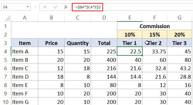
If the formula is copied from E4 to F4, $B4 and $C4 still point to the item’s price and quantity, while E$2 becomes F$2 to pick up the next rate. If it is copied down to E5, the price and quantity references move to row 5, while the rate remains on row 2.
For a closer look, read the mixed-reference example in Absolute, Relative, and Mixed Cell References in Excel. You need not recreate its entire grid; concentrate on why each dollar sign is placed where it is.
Absolute, Relative, and Mixed Cell References in Excel
Read the mixed-reference example by TrumpExcel to connect the commission grid with the rules for copying a formula in two directions.
In “What are Mixed Cell References in Excel?”, start at the instruction to enter a formula in E4 and read the formula breakdown. Focus on what happens to the price, quantity, and rate references when copying across versus down. You can stop before “How to Change the Reference from Relative to Absolute (or Mixed)?”.
For the single-column fee calculation you just built, $J$2 is the clearest choice: it unambiguously means “use this one rate cell wherever I copy the formula.”
Takeaway
A copied Excel formula keeps its calculation, but relative references adjust to the formula’s new position. Use references such as D2 when each result needs inputs from its own row. Use an absolute reference such as $J$2 when every result must draw from one shared cell. Mixed references lock only the row or column when a calculation needs to work across a grid.
Next, you’ll calculate dataset summaries with Excel functions including SUM, AVERAGE, MIN, MAX, and COUNT.