Recommended resources
The freely available resources this lesson will direct you to.
Welcome back. Last lesson, you used formulas to summarize all four finance records. The actual amounts totalled 368, but that number does not tell you which records deserve attention. Today you’ll use sorting to put records in a useful order and filtering to show only records that meet a business condition.
Our question is: Which department-month spending records exceeded budget, and which had the largest overrun? Allow about 35–40 minutes, including time to try the steps in Excel.
Set up a safe inspection area
Use a copy of your data on a new worksheet named Inspection. Keep the header row and every column belonging to each record together. Do not include the summary you built in columns L:N when you select data to sort: it describes the dataset as a whole, rather than one record per row.
If you want an example with results you can check exactly, use this four-row version of the previous lesson’s amounts. In a fresh sheet, place the headers in A1:F1 and the records beneath them. You can enter =D2-E2 in F2 and fill it down to F5.
| department | month | record_id | actual_inr | budget_inr | variance_inr |
|---|---|---|---|---|---|
| Finance | Jan | R01 | 110 | 100 | 10 |
| Operations | Jan | R02 | 95 | 105 | -10 |
| Operations | Feb | R03 | 75 | 80 | -5 |
| Finance | Feb | R04 | 88 | 80 | 8 |
Here, variance_inr is actual minus budget. Because these are spending records, a positive variance means spending exceeded budget. If you use your own workbook instead, your records and answers may differ; keep the same question and use its corresponding columns.
Sort to see the largest overrun first
Sorting rearranges rows. For this question, sort variance_inr from largest to smallest: the largest positive overrun should appear at the top, followed by smaller overruns and then negative variances.
Watch the sorting portion of Excel Sorting and Filtering Data from The Organic Chemistry Tutor. Pay particular attention to what happens when a dataset has several columns: department, month, amounts, and variance must remain attached to the same record.
Excel Sorting and Filtering Data
Watch The Organic Chemistry Tutor’s “Excel Sorting and Filtering Data” for a demonstration of sorting text and numbers while keeping multi-column records intact.
Watch the sorting demonstration. Focus on selecting the complete dataset rather than rearranging one column independently; the horizontal-sorting example is not needed for this lesson.
In Excel, click a cell inside the record range, then choose Data > Filter if your headers do not already have dropdown arrows. Open the variance_inr header arrow and choose Sort Largest to Smallest. For the example, the record IDs should now appear in this order: R01, R04, R03, R02. Check that R04 still has Finance, Feb, actual 88, budget 80, and variance 8. If an amount has become attached to a different record, the sort did not keep whole rows together; return to your untouched copy and sort the complete data range.
The sorted view answers one part of the question immediately: Finance in January has the largest single-record overrun, at 10 INR. It does not yet hide records that were within budget.
Filter to show only relevant records
Filtering works differently from sorting. It temporarily hides rows that fail a condition; it does not delete them. To show overruns, the condition is variance_inr greater than 0.
Watch the short selections from Leila Gharani’s Excel Filter Basics (for quick data analysis). Notice the header controls, the choice of values from a dropdown, and how a filtered view can be cleared.
Excel Filter Basics (for quick data analysis)
Watch Leila Gharani’s “Excel Filter Basics (for quick data analysis)” to see how Excel displays and clears a subset of records.
In enabling filters, watch how header arrows appear. Then watch selecting values from a dropdown. Finally, clearing filters shows how to return to the full view; we will use the header menu to clear a particular condition.
Microsoft Support’s Filter data in a range or table in Excel provides a compact reference for the menu steps and for the distinction between hiding and rearranging rows.
Filter data in a range or table in Excel | Microsoft Support
Read Microsoft Support’s guide to connect the dropdown controls with what a filter actually does to the worksheet.
Under “Filter a range of data,” read the menu steps, from selecting a cell through entering a criterion and confirming it. Under “Learn more about filtering,” read how conditions combine, then filter versus sort. Focus on why an additional filter can leave fewer visible records without removing any from the dataset.
Now open the variance_inr header arrow. Choose Number Filters > Greater Than, enter 0, and select OK. The screenshot below shows where Excel places Number Filters; it highlights Between, but Greater Than is the option for our overrun question.
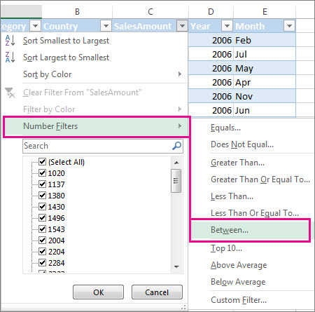
Only R01 and R04 should remain visible in the example. R02 and R03 still exist; their negative variances simply do not meet the condition. A dropdown may offer Text Filters instead of Number Filters if a column’s values are stored as text—an indication to inspect the data rather than assume the comparison worked.
Narrow the question, then restore the full view
Suppose the manager asks a more specific question: Which February records exceeded budget? Keep the variance_inr > 0 filter and open the month dropdown. Deselect other months so that only Feb is checked, then select OK. Both conditions now apply. In the example, R04 (Finance, Feb, overrun 8 INR) is the only visible record.
These Jan and Feb entries are text labels, not Excel dates. Selecting Feb from the value list is appropriate here; a Date Filters menu requires a column containing actual date values.
When you finish inspecting, use each filtered column’s dropdown and choose Clear Filter From…. Clear the month filter first: the two overruns reappear. Clear the variance filter next: all four records reappear. Clearing filters does not undo the sort; the records remain ordered by variance. If you need the example’s original order again, sort record_id from A to Z. On your own data, use an original-order identifier only if you have one; otherwise, retain the untouched copy.
One final distinction matters after filtering: the ordinary SUM formula from last lesson still includes rows hidden by a filter. For the example, =SUM(D2:D5) remains 368, even while only two overrun rows are visible. Do not label that result “total of visible overruns.”
Takeaway
Sort when order helps you spot a record, such as the largest overrun. Filter when you need to inspect records meeting a condition, such as positive variance in February. Keep entire records together, check the visible rows against the question, and clear filters when you need the full dataset again.
Next, you’ll inspect the spreadsheet for missing values, duplicates, inconsistent labels, and invalid values—problems that can make a sort or filter give a misleading view.