Calculating Masking and Retention Probabilities

Recommended resources

The freely available resources this lesson will direct you to.

Hello! Last time, you saw that forward corruption replaces text tokens with [MASK], while a learned denoiser tries to predict what belongs in the gaps. Today we will answer a narrower question: at a chosen noise level, how likely is each token to be hidden? This calculation will become the masking rule in your later Colab implementation.

Allow about 15–20 minutes for the reading and lesson.

A schedule turns a noise level into a probability

Imagine the clean sequence the cat sleeps .. We assign it a noise level $t$ , usually between $0$ (clean) and $1$ (fully masked). A masking schedule tells us how much of the original text should remain visible at that level.

Read the opening explanation of the forward process in How to Build a Diffusion Language Model by the Kuleshov Group.

How to Build a Diffusion Language Model | Kuleshov Group

Read this for the definition of the signal level and its relationship to the chance of masking a token.

In the forward-process discussion immediately above the “Reverse process” heading, read the schedule explanation, beginning “The key challenge is deciding what ‘noisy’ should mean.” Then read the first figure caption beneath the diagram of the clean and partially masked sequences. Stop there; the following paragraph about a Markov chain concerns transitions between levels, which we will examine next time.

The article calls the schedule value $α_{t}$ the signal level. It means the probability that an individual clean token survives corruption at level $t$ . Since a valid position has only two possible outcomes—its original token or [MASK]—the probabilities must add to one:

P (retain a valid token at t) = α_{t}, P (mask a valid token at t) = 1 - α_{t} .

At $t = 0$ , the schedule gives $α_{0} = 1$ : every token remains visible. At $t = 1$ , it gives $α_{1} = 0$ : every valid token is masked. Between those endpoints, the schedule determines the probabilities.

Noise level and masking probability are not necessarily the same number. They coincide for one common choice, the linear schedule $α_{t} = 1 - t$ . With that schedule, $P (mask) = t$ . For any other schedule, calculate $α_{t}$ first rather than assuming that $t$ itself is the masking probability.

Calculate the probabilities, then interpret the result

Suppose we choose the linear schedule and set $t = 0.3$ . Then:

α_{0.3} = 1 - 0.3 = 0.7, P (mask) = 1 - 0.7 = 0.3.

Each valid position in the cat sleeps . has a 70% chance of retaining its original token and a 30% chance of becoming [MASK]. The rate applies to every position, but the random decisions need not have the same outcome. One draw might give the [MASK] sleeps .; another might give [MASK] cat sleeps [MASK].

There are four valid tokens, so the expected number masked is $4 (0.3) = 1.2$ . You cannot mask exactly 1.2 tokens in a particular sequence. The expectation describes what you would average over many independently corrupted copies; it is not an instruction to select exactly one token.

Now change only the schedule. Suppose $α_{t} = 1 - t^{2}$ , and choose $t = 0.6$ . The schedule gives:

α_{0.6} = 1 - (0.6)^{2} = 0.64.

Thus each valid token is retained with probability $0.64$ and masked with probability $0.36$ —not $0.6$ . The noise level identifies a point on the schedule; the schedule supplies the actual probabilities.

“Each valid token” excludes padding

Later, your batches will contain [PAD] positions so that examples can share a fixed length. Padding is not part of the clean text we want the denoiser to recover. For example:

the  cat  sleeps  .  [PAD]  [PAD]

At a level where $α_{t} = 0.7$ , each of the first four positions has a $0.3$ masking probability. The two [PAD] positions are ineligible for corruption: they stay [PAD], not [MASK]. So the expected masked count is $4 (0.3) = 1.2$ , not $6 (0.3) = 1.8$ .

In code, the idea will be to draw random masking decisions and apply them only where a position is valid. For now, keep the distinction between the schedule’s probability and a position’s eligibility: a schedule tells you how likely masking is; a validity mask tells you where it may happen.

Reading the forward-process picture

The image below shows a clean sequence at the top and increasingly masked versions below it. As the signal level $α_{t}$ decreases, fewer original tokens remain visible.

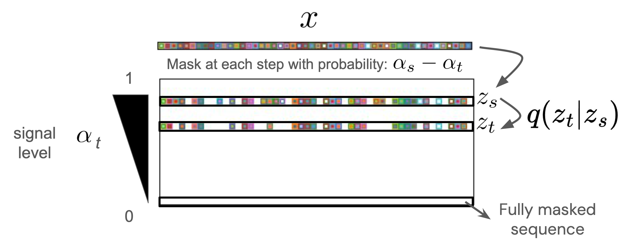
A clean token sequence is progressively replaced by blank mask positions as its retention probability decreases from 1 to 0. The intermediate rows illustrate possible random outcomes, not an exact required number of masks.

One detail in the image is worth setting aside carefully. Its label $α_{s} - α_{t}$ describes the drop in overall retention probability between two levels. It is not, by itself, the probability of masking a token conditional on that token still being visible at the earlier level. We will work through that distinction when we trace an entire forward trajectory in the next lesson. For today’s calculation directly from clean text at level $t$ , use $α_{t}$ for retention and $1 - α_{t}$ for masking.

Takeaway

A masking schedule converts a noise level $t$ into a retention probability $α_{t}$ . For every valid token, the masking probability is its complement, $1 - α_{t}$ ; padding stays untouched. These are per-token probabilities, so a short sample’s actual masked fraction can differ from the scheduled rate.

Next, we will follow the same sequence through several noise levels and see how progressive masking relates to sampling a corrupted sequence directly from the clean one.