Recommended resources
The freely available resources this lesson will direct you to.
Hello! Last time, you compared a model that extends text from left to right with one that fills masked positions across a whole sequence. Today we will look behind that second picture: how do we make a noisy text example, and what does the model actually learn to undo? We will keep the theory light and use the same idea that you will later implement in PyTorch.
Allow about 15–20 minutes for the lesson, including the short video clips.
First, what “noise” means for a diffusion model
A diffusion model has two distinct jobs. The forward process takes a clean training example and corrupts it according to a rule we choose. The reverse process uses a learned model to make corrupted data look more like clean data. Only the reverse process needs to learn.
For an image, the corruption can be additive Gaussian noise: pixel values are continuous numbers, so we can mix them with random numerical values. With enough corruption, a recognizable image becomes something like static. A denoiser trained on noisy images can then be used repeatedly, starting from noise, to generate an image.
Watch the image example and the beginning of the text comparison in Diffusion Language Models: The Next Big Shift in GenAI by Jia-Bin Huang.
Diffusion Language Models: The Next Big Shift in GenAI
Jia-Bin Huang’s video gives a compact visual account of Gaussian corruption, then explains why applying that operation directly to text token IDs is problematic.
Watch image noising for the forward and learned reverse processes. Then watch token IDs for the distinction between discrete token IDs and continuous embeddings. You can stop before the discussion of other text-generation strategies.
The important distinction is what kind of object is being corrupted. Gaussian noise is meaningful for numerical image values. But if one token has ID 17 and another has ID 18, their numerical proximity does not mean their words are similar. Adding a small random number to 17 does not produce a slightly corrupted word.
It is possible to apply Gaussian diffusion to continuous token embeddings rather than IDs. That is a different design. In this course, we will work directly with discrete tokens and use a simpler corruption rule: replace a token with [MASK].
Forward corruption: hide tokens, do not perturb them
Consider a clean four-token training example:
the cat sleeps .
At one chosen noise level, a forward masking rule might produce:
the [MASK] sleeps [MASK]
At a stronger level, it might produce:
[MASK] [MASK] sleeps [MASK]
Each surviving token is still exactly itself; each hidden token is replaced by the special mask symbol. Nothing halfway between cat and [MASK] appears in the sequence. The noise level controls how likely positions are to be hidden, not how much their token IDs change. We will calculate those probabilities in the next lesson.
For the particular absorbing-mask forward process we will use, a position that becomes masked stays masked as corruption continues. This describes the forward training rule. It does not mean a generator can never reconsider one of its predicted tokens; that depends on the sampling method.
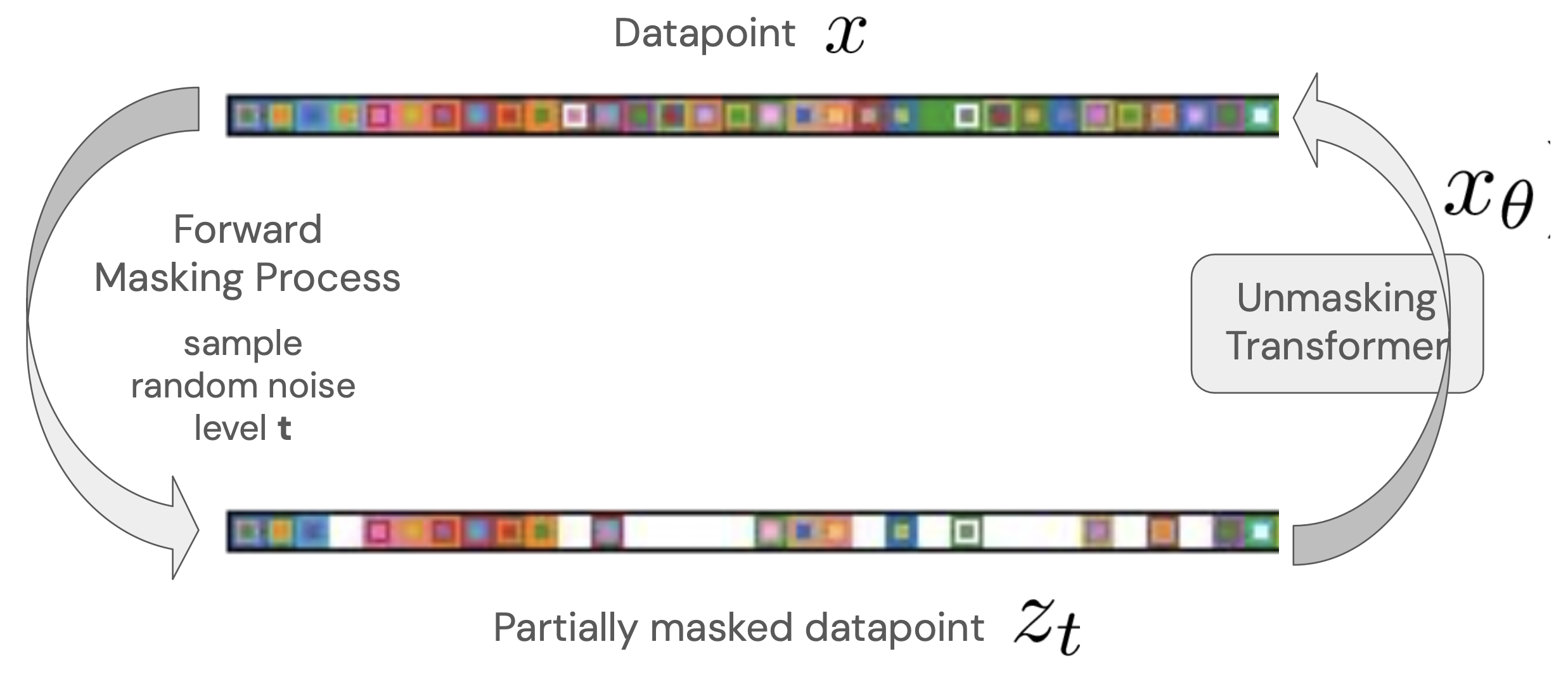
The diagram’s upper sequence is available when creating a training example. Its lower sequence is the corrupted input given to the model. The hiding rule is specified by us; it does not have to be discovered by the transformer.
Watch the video’s discrete-text example now. Where it describes tokens becoming masked over successive phases, read that as the forward corruption process; denoising runs in the opposite direction.
Diffusion Language Models: The Next Big Shift in GenAI
The same video illustrates a mask as a discrete noise state and shows how a trained model can fill masked positions during generation.
Watch mask state for the discrete alternative to Gaussian noise. Continue through forward masking, then reverse filling. Focus on the difference between choosing to hide a known token and predicting an unknown token.
When the video shows a mixture of a clean-token state and a mask state, that mixture describes probabilities: a draw yields either the original token or [MASK]. It is not an intermediate, fractional word.
Learned reverse denoising: make a prediction, then reveal
During training, we know that the hidden tokens in the [MASK] sleeps [MASK] were cat and .. We can ask a model to assign probabilities to possible original tokens at those positions and train it to favor the known answers. It can use visible context on both sides of a mask: the and sleeps, for example, both inform its prediction for the second position.
During generation, that original sentence is not available. We instead start with a chosen number of masked slots:
[MASK] [MASK] [MASK] [MASK]
The trained denoiser proposes token distributions for masked positions. A sampling procedure selects predictions to reveal, passes the partly filled sequence back to the denoiser, and repeats. A possible result could be the dog sleeps .; generation is not an attempt to recover the particular training sentence the cat sleeps ..
This is why “reverse” needs a little care. Forward corruption is a known random rule, but masking destroys information: the [MASK] sleeps . could have come from many different sentences. The model cannot mechanically invert a mask. It learns from examples which completions are plausible and uses those predictions to guide generation. In the simple sampler we first build, revealed tokens will stay fixed; other samplers can reconsider tentative predictions.
The two kinds of diffusion therefore share a blueprint but differ in their working material:
| Gaussian diffusion | Masked text diffusion | |
|---|---|---|
| Data being corrupted | Continuous values | Discrete tokens |
| Forward corruption | Mix in numerical noise | Replace selected tokens with [MASK] |
| Learned reverse task | Estimate cleaner values or added noise | Predict plausible original tokens at masked positions |
| Starting point for generation | Numerical noise | Masked token slots |
Takeaway
Forward masking creates the training problem; learned unmasking supplies the generative ability. Unlike Gaussian image noise, mask corruption keeps text in the discrete vocabulary: a position contains a token or [MASK]. At generation time, the clean answer is unknown, so repeated model predictions—not an exact reversal of a known sentence—produce new text.
Next, we will make “how noisy?” precise by calculating the probabilities that each valid token remains visible or becomes masked.