Monopoly: Profit Maximization

Introduction

Welcome back! In our previous lesson, we established that a monopoly exists because of high barriers to entry, which grant the firm market power. This makes the monopolist a price maker, facing a downward-sloping demand curve for its product.

But how does a firm with this power decide what price to charge and how much to produce? Simply having the power to set any price doesn't mean any price is a good choice. In this lesson, we will determine how a monopolist finds its profit-maximizing price and output.

You'll discover that while the fundamental rule of profit maximization—producing where marginal revenue equals marginal cost (MR = MC)—is the same one we saw in perfect competition, the outcome is vastly different. The key distinction lies in the relationship between price and marginal revenue, which we'll explore in detail.

1. The Monopolist's Marginal Revenue

For a perfectly competitive firm, marginal revenue is simple: it equals the market price (MR = P). This is because the firm can sell as much as it wants at the going market rate.

A monopolist's situation is different. Because it faces the entire downward-sloping market demand curve, if it wants to sell more, it must lower its price. Crucially, it must lower the price not just for the additional unit but for all units it sells. This leads to two opposing effects on total revenue:

1. The Output Effect: Selling one more unit increases total revenue by the price of that unit.
2. The Price Effect: To sell that extra unit, the firm must lower its price, which reduces the revenue earned on all the units it was already selling.

Because of this negative price effect, a monopolist's marginal revenue from selling an additional unit is always less than the price it charges (MR < P).

Let's watch a video that explains this concept and then shows how to apply the profit-maximization rule graphically.

2. The Profit-Maximizing Decision: A Graphical Approach

As the video demonstrated, finding the monopolist's optimal price and quantity is a systematic, two-step graphical process, guided by the rule MR = MC.

Let's break it down with a clear diagram.

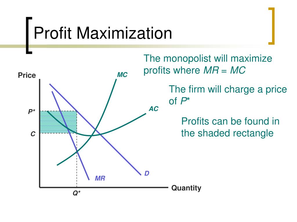
Here is the procedure:

1. Find the Profit-Maximizing Quantity (Q*): Locate the point where the Marginal Revenue (MR) curve intersects the Marginal Cost (MC) curve. This intersection determines the optimal quantity to produce. Why? Because for every unit up to this point, the additional revenue from selling it (MR) was greater than or equal to the additional cost of producing it (MC).
2. Find the Profit-Maximizing Price (P*): Once you have Q*, do not take the price from the MR=MC intersection. Instead, trace a vertical line from Q* up to the Demand (D) curve. The demand curve tells you the highest price consumers are willing to pay for that specific quantity. From that point on the demand curve, trace a horizontal line to the vertical price axis to find P*.
3. Calculate the Profit: At quantity Q*, find the corresponding average cost on the Average Cost (AC) curve. The monopolist's total economic profit is the shaded rectangular area, calculated as: $$\text{Profit}=(\text{Price}-\text{Average Cost})\times \text{Quantity}=(P^{\ast }-C)\times Q^{\ast }$$

This graphical method is the cornerstone of analyzing monopoly behavior. Always remember the two-step process: first find quantity at MR=MC, then find price on the demand curve.

3. An Analytical Approach to Profit Maximization

Given your background, you'll likely appreciate that we can also solve this problem using a more formal mathematical approach. This method yields the same result as the graphical analysis but allows for precise calculations.

Let's explore a textbook section that walks through this process.

The reading confirms that the goal is to maximize the profit function, $\pi =TR-TC$. The process, as outlined in the text, involves these steps:

1. Define the Profit Function: Start with the equations for demand and total cost.

   • Inverse Demand: $P=f(Q)$
   • Total Revenue: $TR=P\times Q=f(Q)\times Q$
   • Total Cost: $TC=g(Q)$
   • Profit: $\pi (Q)=TR(Q)-TC(Q)$

2. Find the Maximum: To find the quantity (Q) that maximizes profit, we take the first derivative of the profit function with respect to Q and set it to zero.

   $$\frac{d\pi }{dQ}=\frac{d(TR)}{dQ}-\frac{d(TC)}{dQ}=0$$

3. Apply the MR = MC Rule: You'll recognize that $\frac{d(TR)}{dQ}$ is the definition of Marginal Revenue (MR) and $\frac{d(TC)}{dQ}$ is the definition of Marginal Cost (MC). So, the profit-maximization condition is simply:

   $$MR-MC=0\text{or}MR=MC$$

Let's apply this to the example from the reading:

• Inverse Demand: $P=100-Q$
• Total Cost: $TC=10Q$, which means Marginal Cost (MC) is constant at 10.

First, we find Total Revenue (TR) and Marginal Revenue (MR):

• $TR=P\times Q=(100-Q)Q=100Q-Q^2$
• $MR=\frac{d(TR)}{dQ}=100-2Q$

Next, we set MR = MC:

• $100-2Q=10$
• $90=2Q$
• $Q^{\ast }=45$

Finally, we find the price by plugging $Q^{\ast }$ back into the demand equation:

• $P^{\ast }=100-45=55$

The result is a profit-maximizing quantity of 45 million ounces sold at a price of $55 per ounce, exactly as derived in the text. This analytical method provides a precise and powerful way to solve for the monopolist's optimal strategy.

Conclusion

In this lesson, we have moved from understanding why a monopolist has market power to analyzing how it uses that power. We have built a complete model to determine its profit-maximizing price and output.

Here are the essential takeaways:

• A monopolist's marginal revenue (MR) is always less than its price (P) because it must lower the price on all units to sell an additional unit.
• The profit-maximization rule is to produce the quantity (Q*) where marginal revenue equals marginal cost (MR = MC).
• The profit-maximizing price (P*) is found by taking Q* and going up to the demand curve.
• This problem can be solved both graphically (by finding the intersection of the MR and MC curves) and analytically (by taking the derivative of the profit function and setting it to zero).

We now know how a monopolist behaves. But is this behavior good for society? By charging a price higher than marginal cost and producing less than a competitive market would, the monopolist creates a different outcome. In our next lesson, we will evaluate the efficiency of monopoly by calculating the deadweight loss it creates, providing a crucial tool for comparing market structures.