Mean-Field Critical Exponents of the Ising Model

Hello and welcome back to our study of mean-field theory!

In the previous lesson, we made a significant breakthrough. By solving the mean-field self-consistency equation, we uncovered its most important prediction: the existence of a continuous phase transition at a critical temperature $T_c$. We analyzed the behavior just below this transition and found that the spontaneous magnetization—our order parameter—vanishes as $m\propto (T_c-T{)}^{1/2}$. This gave us our first critical exponent, $\beta =1/2$.

Today, we will complete our characterization of the mean-field critical point. The behavior of a system near criticality is described by a whole set of exponents, each governing how a specific physical quantity responds or diverges. Our objective is to calculate the full set of mean-field critical exponents ($\alpha$, $\beta$, $\gamma$, $\delta$) for the Ising model.

1. The Language of Criticality: Defining the Exponents

Critical exponents provide a universal language to describe the nature of a phase transition. They quantify the singular, or non-analytic, behavior of thermodynamic quantities as we approach the critical point. Let's formally define the exponents we will calculate today. We'll use the reduced temperature, $t=(T-T_c)/T_c$, which is a dimensionless measure of the distance from the critical temperature.

• Specific Heat ($\alpha$): Describes the singularity in the specific heat at zero field.
  $C_h\propto |t{|}^{-\alpha }(h=0)$
• Spontaneous Magnetization ($\beta$): Describes how the order parameter vanishes as $T\to T_c$ from below.
  $m_0\propto (-t{)}^{\beta }(h=0,t<0)$
• Isothermal Susceptibility ($\gamma$): Describes the divergence of the magnetic susceptibility at zero field.
  ${\chi }_T={\left(\frac{\partial m}{\partial h}\right)}_T\propto |t{|}^{-\gamma }(h=0)$
• Critical Isotherm ($\delta$): Describes the relationship between magnetization and field exactly at the critical temperature.
  $h\propto |m{|}^{\delta }\text{sgn}(m)(t=0)$

We've already found $\beta$, but we will re-derive it along with the others from a single, powerful starting point.

2. The Equation of State Near Criticality

To find all the exponents, we need an approximate equation relating $m$, $h$, and $t$ that is valid near the critical point ($t\to 0,h\to 0,m\to 0$). In the last lesson, we started this by expanding the self-consistency equation $m=\tanh (\beta (h+Jzm))$. A more careful expansion reveals a master equation that contains all the physics we need.

The following resource performs this expansion and derives the key equation of state.

As the document shows, after expanding the hyperbolic tangent and keeping the leading order terms in $m$ and $t$, we arrive at the approximate equation of state:
$h\approx k_B{T}_c\left(\frac{T-T_c}{T_c}m+\frac{1}{3}{m}^3\right)$
Or, using our reduced temperature $t=(T-T_c)/T_c$:
$h\approx Atm+B{m}^3$
where $A=k_B{T}_c$ and $B=k_B{T}_c/3$ are positive constants. This simple cubic equation is remarkably powerful. It's an example of what is known as a Landau free energy expansion, a topic we will explore in great detail in a future module. For now, let's use it to extract the exponents.

3. Calculating the Exponents

We will now systematically apply the definitions of the critical exponents to our approximate equation of state, $h\approx Atm+B{m}^3$. The resource you just read, LINK, walks through these calculations. Let's tackle them one by one.

Exponent $\delta$: The Critical Isotherm

First, let's find $\delta$. This exponent is defined along the critical isotherm, where $T=T_c$, which means $t=0$.

As the resource shows, when we set $t=0$, our equation of state simplifies dramatically to:
$h\approx B{m}^3$
Comparing this to the definition $h\propto m^{\delta }$, we immediately identify the mean-field value:
$\delta =3$

Exponent $\beta$: Spontaneous Magnetization

Next, let's re-derive $\beta$. This involves looking for spontaneous magnetization ($m_0\ne 0$) in the absence of an external field ($h=0$) for temperatures below $T_c$ ($t<0$).

Setting $h=0$, our equation becomes $0\approx Atm+B{m}^3$. This has two types of solutions:

1. $m=0$ (the paramagnetic solution)
2. $At{m}_0+B{m}_0^3=0⟹m_0^2=-\frac{A}{B}t$

The second solution is only real if $t<0$ (i.e., $T<T_c$), which is exactly what we expect for spontaneous magnetization. It gives:
$m_0=\sqrt{-\frac{A}{B}t}\propto (-t{)}^{1/2}$
Comparing this to the definition $m_0\propto (-t{)}^{\beta }$, we find the mean-field value:
$\beta =1/2$
This confirms the result from our previous lesson.

Exponent $\gamma$: Magnetic Susceptibility

Now for the susceptibility, ${\chi }_T=(\partial m/\partial h{)}_T$ as $h\to 0$. It's easier to first calculate $(\partial h/\partial m{)}_T$ from our equation of state and then take the reciprocal.

Differentiating $h\approx Atm+B{m}^3$ with respect to $m$ gives:
$\frac{\partial h}{\partial m}\approx At+3B{m}^2$
So, ${\chi }_T=(\frac{\partial m}{\partial h}{)}_T\approx \frac{1}{At+3B{m}^2}$. We now evaluate this in the limit $h\to 0$:

• For $T>T_c$ ($t>0$): At $h=0$, the stable solution is $m=0$. The susceptibility is ${\chi }_{+}\approx \frac{1}{At}\propto t^{-1}$.
• For $T<T_c$ ($t<0$): At $h=0$, the stable solution is $m_0^2=-\frac{A}{B}t$. Substituting this in gives ${\chi }_{-}\approx \frac{1}{At+3B(-\frac{A}{B}t)}=\frac{1}{At-3At}=\frac{1}{-2At}\propto (-t{)}^{-1}$.

In both cases, the susceptibility diverges as $|t{|}^{-1}$. Therefore, the mean-field exponent is:
$\gamma =1$
The resource also notes that the ratio of the amplitudes, ${\chi }_{+}/{\chi }_{-}$, approaches a universal constant (2 in this case) at $T_c$. This is another characteristic feature of critical phenomena.

Exponent $\alpha$: Specific Heat

Finally, we come to $\alpha$, the specific heat exponent. This is the most involved calculation as it requires finding the free energy first. The Helmholtz free energy density, $f(T,m)$, can be found by integrating the equation of state: $f(T,m)-f(T,0)={\int }_0^{m}h(m^{\prime })d{m}^{\prime }$. The equilibrium Gibbs free energy is then the value of $f$ at the magnetization $m^{\ast }$ that minimizes it. The specific heat is then found from the second derivative of the Gibbs free energy with respect to temperature.

Following the steps in the document:

1. The Helmholtz free energy has the form $f(m,T)\approx f_0(T)+\frac{1}{2}At{m}^2+\frac{1}{4}B{m}^4$.
2. The equilibrium magnetization $m^{\ast }$ minimizes this free energy.
   • For $T>T_c$, $m^{\ast }=0$.
   • For $T<T_c$, $m^{\ast }=m_0$ where $m_0^2=-At/B$.
3. The equilibrium Gibbs free energy is $g(T)=f(m^{\ast },T)$.
   • For $T>T_c$, $g(T)=f_0(T)$.
   • For $T<T_c$, substituting $m_0$ gives $g(T)=f_0(T)-\frac{A^2}{4B}{t}^2=f_0(T)-\frac{A^2}{4B{T}_c^2}(T-T_c{)}^2$.
4. The specific heat is $c\propto -T({\partial }^{2}g/\partial T^2)$.
   • For $T>T_c$, the singular part is zero.
   • For $T<T_c$, the second derivative of the $(T-T_c{)}^2$ term is a constant.

This means the specific heat does not diverge at $T_c$. Instead, it has a finite jump discontinuity. A function that has a finite value or a finite jump does not have a power-law divergence. For the form $c\propto |t{|}^{-\alpha }$ to remain finite as $t\to 0$, the exponent must be zero.
$\alpha =0$

Summary and a Look Ahead

We have successfully derived the full set of classical, mean-field critical exponents for the Ising model.

Key Takeaways:

• A simple polynomial equation of state, $h\approx Atm+B{m}^3$, derived from the mean-field approximation, contains all the information needed to find the critical exponents.
• The mean-field critical exponents for the Ising model are:
  • $\alpha =0$ (finite jump in specific heat)
  • $\beta =1/2$ (order parameter)
  • $\gamma =1$ (susceptibility)
  • $\delta =3$ (critical isotherm)
• These exponents are "universal" within mean-field theory—they are independent of the microscopic details like lattice dimension or structure.

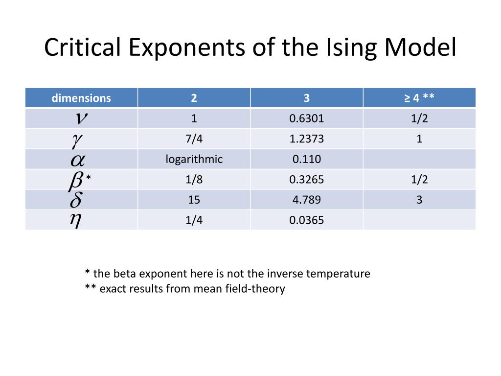
Here is a summary table from another resource that aligns with our findings. The document the infinite range ising model... derives these same exponents using a slightly different formalism (the infinite-range model, for which mean-field theory is exact) but arrives at the identical results.

Preview of the Next Lesson:
We have now fully characterized the mean-field solution for the Ising model. But how good is this approximation? The image above hints that it's not the full story, especially in lower dimensions. In our next lesson, we will begin to answer the crucial question: When does mean-field theory work, and when does it fail? We will introduce the concepts of fluctuations and dimensionality, which are the keys to understanding the limitations of this powerful but approximate theory.