Magnetization Near the Critical Point: Graphical and Analytical Solutions

Recommended resources

The freely available resources this lesson will direct you to.

Hello! Welcome back to our module on mean-field theory.

In our last lesson, we derived the central equation of the mean-field approximation for the Ising model: the self-consistency equation for magnetization $m$ . We found that by replacing the fluctuating influence of neighboring spins with a static, average "molecular field," the magnetization must satisfy:

$m = tanh (β (h + J z m))$

where $h$ is the external field energy, $z$ is the number of nearest neighbors, and $β = 1/ (k_{B} T)$ . This equation, while simple in appearance, holds the key to understanding how a collective phenomenon like a phase transition can emerge from simple microscopic interactions.

Today, we will solve this equation. Our goal is to see how this single, transcendental equation predicts a phase transition and to characterize the behavior of the system near this transition. Specifically, we will fulfill the learning outcome: Solve the self-consistency equation for magnetization graphically and analytically near the critical point.

1. Graphical Solution: The Emergence of a Transition

An analytical solution for $m$ is generally not possible, but we can gain immense physical insight by solving the equation graphically. Let's start with the most interesting case: the possibility of magnetism without an external field, known as spontaneous magnetization. We set the external field $h = 0$ , simplifying our equation to:

$m = tanh (β J z m)$

To find the solutions for $m$ , we can plot the left-hand side, $y = m$ , and the right-hand side, $y = tanh (β J z m)$ , on the same graph. The points where the curves intersect represent the physically allowed values for the magnetization.

The following video provides an excellent visual demonstration of this graphical solution and its consequences.

Lecture 42: Mean Field Theory

Let's walk through the graphical solution. The following video from NPTEL IIT Kharagpur clearly demonstrates how to plot the two sides of the self-consistency equation and interpret the intersections.

Please watch from 21:04 to 27:16. The presenter analyzes how the number of solutions changes with temperature. Pay close attention to the role of the slope of the tanh function at the origin. This slope is the key to identifying the critical temperature.

As the video explains, the behavior of the system hinges on the slope of $f (m) = tanh (β J z m)$ at $m = 0$ . The slope of the line $y = m$ is always 1. For the hyperbolic tangent function $tanh (a x)$ , the slope at $x = 0$ is $a$ . In our case, this slope is $β J z$ .

This leads to three distinct regimes:

High Temperature ( $β J z < 1$ ):
The initial slope of the $tanh$ curve is less than 1. The straight line $y = m$ only intersects the $tanh$ curve at $m = 0$ . This means the only possible state is one with no spontaneous magnetization. The system is in a paramagnetic phase. Thermal energy is too high for the spin interactions to establish long-range order.
Low Temperature ( $β J z > 1$ ):
The initial slope of the $tanh$ curve is greater than 1. This leads to three intersection points: one at $m = 0$ and two symmetric solutions at $\pm m_{0}$ , where $m_{0} > 0$ . These non-zero solutions correspond to a state of spontaneous magnetization. The system is in a ferromagnetic phase.
Critical Temperature ( $β_{c} J z = 1$ ):
This is the threshold case where the initial slope of the $tanh$ curve is exactly 1. This condition defines the critical temperature, $T_{c}$ .
$\frac{1}{k _{B} T _{c}} J z = 1 ⟹ k_{B} T_{c} = J z$
Above $T_{c}$ , there is no spontaneous order; below $T_{c}$ , the system spontaneously magnetizes. This is a second-order phase transition.

Test your understanding!

Consider a 2D Ising model on a triangular lattice. What is the mean-field prediction for the critical temperature $T_{c}$ in this case? Express your answer in units of $J / k_{B}$ .

Show answer

In a triangular lattice, each site is surrounded by 6 nearest neighbors, so the coordination number is $z = 6$ .
The critical temperature is given by the condition $k_{B} T_{c} = J z$ .
Substituting $z = 6$ , we get $k_{B} T_{c} = 6 J$ , or $T_{c} = 6 J / k_{B}$ .

2. Analytical Solution Near the Critical Point

The graphical method gave us the qualitative picture. Now, let's zoom in on the behavior just below the critical temperature $T_{c}$ . Near $T_{c}$ , the magnetization $m$ will be very small. This allows us to use a Taylor expansion for the hyperbolic tangent function:
$tanh (x) \approx x - \frac{x ^{3}}{3} + \dots$
Our self-consistency equation $m = tanh (β J z m)$ becomes:
$m \approx (β J z) m - \frac{( β J z ) ^{3} m ^{3}}{3}$
This equation has the trivial solution $m = 0$ . To find the non-zero solutions corresponding to the ferromagnetic state, we can divide by $m$ (assuming $m \neq = 0$ ):
$1 \approx β J z - \frac{( β J z ) ^{3} m ^{2}}{3}$
Rearranging to solve for $m^{2}$ :
$m^{2} \approx 3 \frac{β J z - 1}{( β J z ) ^{3}}$
We are interested in the behavior as $T \to T_{c}$ from below. Let's express $β J z$ in terms of temperatures. Using $k_{B} T_{c} = J z$ , we have $β J z = \frac{J z}{k _{B} T} = \frac{T _{c}}{T}$ . Substituting this in:
$m^{2} \approx 3 \frac{T _{c} / T - 1}{( T _{c} / T ) ^{3}} = 3 \frac{T _{c} - T}{T} (\frac{T}{T _{c}})^{3}$
As $T \to T_{c}$ , the ratio $T / T_{c}$ approaches 1. So, for temperatures very close to $T_{c}$ , we get:
$m^{2} \propto (T_{c} - T)$
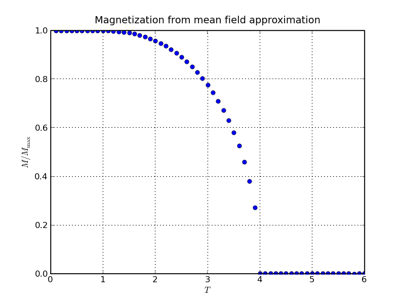
This implies that for $T < T_{c}$ , the spontaneous magnetization behaves as:
$m (T) \propto T_{c} - T$
This result defines the critical exponent $β$ (not to be confused with the thermodynamic beta!), which describes how the order parameter vanishes as the critical point is approached. We find that mean-field theory predicts $β = 1/2$ .

The following document provides a concise summary of this analytical derivation.

[PDF] Mean_Field.pdf - KFUPM

To solidify the analytical steps, let's consult a written resource. This PDF provides a compact derivation of the magnetization behavior near T_c.

Please refer to page 5 of the document. Start from the line 'At H = 0, one finds...'. Follow the steps that lead to the expression for m for T < T_c, showing that it behaves as (T_c - T)^(1/2). This derivation gives us the critical exponent β.

The curve showing magnetization as a function of temperature summarizes our findings perfectly.

Magnetization from Mean Field Approximation — The temperature dependence of the spontaneous magnetization $m$ as predicted by the mean-field approximation. For temperatures $T > T_c$, the only solution is $m=0$ (paramagnetic phase). For $T < T_c$, a non-zero magnetization appears spontaneously, growing as $T$ decreases. The shape of the curve near the critical temperature $T_c$ is precisely what we derived analytically: $m \propto (T_c-T)^{1/2}$.

3. Stability and Spontaneous Symmetry Breaking

Below $T_{c}$ , we found three solutions: $m = 0$ and $\pm m_{0}$ . A crucial question remains: which solution does the system choose? The $m = 0$ solution is in fact unstable, while the $\pm m_{0}$ solutions are stable.

A powerful way to visualize this is to consider the effect of an infinitesimally small external field, $h$ . This field will break the up/down symmetry of the Hamiltonian. If $h$ is positive, it will slightly favor the "up" spin state.

Leonard Susskind provides a masterfully intuitive explanation of how this tiny field resolves the ambiguity in the graphical solution.

Statistical Mechanics Lecture 9

Why is the m=0 solution unstable below T_c? Introducing a tiny external field provides a clear answer and a beautiful illustration of spontaneous symmetry breaking.

Please watch the segment from 1:20:19 to 1:28:40. Professor Susskind modifies the graphical solution by adding a small external field term. Observe how this small perturbation breaks the symmetry of the problem and makes it clear why the system must choose one of the magnetized branches, even as the field is taken to zero.

As the video shows, any non-zero field $h$ , no matter how small, makes one of the magnetized solutions the only stable option. In a real physical system, there are always stray fields. Taking the limit $h \to 0$ after solving the problem leads to a definite magnetized state. This process, where the ground state of a system has less symmetry than the underlying laws that govern it, is a profound concept known as spontaneous symmetry breaking.

Conclusion

In this lesson, we have brought the mean-field equation to life. By solving it, we have uncovered the core prediction of mean-field theory: the existence of a continuous phase transition.

Key Takeaways:

The self-consistency equation can be solved graphically, revealing a critical temperature $T_{c} = J z / k_{B}$ that separates a high-temperature paramagnetic phase ( $m = 0$ ) from a low-temperature ferromagnetic phase ( $m \neq = 0$ ).
An analytical solution near the critical point shows that the spontaneous magnetization grows as $m \propto (T_{c} - T)^{1/2}$ , yielding the mean-field critical exponent $β = 1/2$ .
The choice between the two degenerate magnetized states ( $\pm m_{0}$ ) below $T_{c}$ is an example of spontaneous symmetry breaking, a process that can be visualized by considering the effect of an infinitesimal external field.

Preview of the Next Lesson:
We have now extracted the critical temperature and the exponent $β$ . But this is just the beginning. The self-consistency equation contains all the information about the system's behavior near the critical point. In our next lesson, we will use it to calculate the full set of mean-field critical exponents: $α$ (specific heat), $γ$ (susceptibility), and $δ$ (critical isotherm). This will complete our characterization of the mean-field critical point.