Visualizing Recursive Call Trees

Welcome to the second lesson on recursion. In our last session, we built a solid foundation by breaking down recursive functions into three core components: the explicit state, the base case, and the progress step. This provided a structured way to think about and write recursive code.

Today, we're going to pull back the curtain and see what's actually happening when a recursive function executes. Our goal is to demystify the "magic" of recursion by learning how to trace its flow of calls and returns. You'll learn to build a call tree, a powerful visual tool for understanding, debugging, and ultimately analyzing any recursive algorithm. This skill will be indispensable as we move on to more complex recursive patterns.

How Recursion Works: The Call Stack

As a developer with years of experience, you're likely familiar with the concept of the function call stack. Every time a function is called, the program creates an "execution context" (or stack frame) containing that function's local variables and parameters, and pushes it onto the call stack. When a function returns, its frame is popped off the stack.

Recursive functions use this very same mechanism. The key difference is that multiple frames for the same function can exist on the stack simultaneously, each with different parameter values.

Let's get a more formal understanding of this process. The following reading from Launch School's "Advanced DSA" book provides an excellent explanation, first with non-recursive functions and then applying the same logic to the factorial function we saw in the last lesson.

The key takeaway is this: the call stack grows with each recursive call until a base case is reached. At that point, the stack begins to "unwind" as each function call receives a return value from the call it made, completes its own computation, and returns its result to the caller above it in the stack.

From Call Stack to Call Tree

While the call stack shows us the precise, moment-to-moment state of execution, it can be difficult to see the overall structure of the computation. A more intuitive and powerful visualization is the recursion tree, or call tree.

In a call tree:

• Each node represents a specific function call with its arguments (e.g., factorial(4)).
• An edge from a parent node to a child node means the parent function made a direct recursive call to the child function.

For a function like factorial(n), which only makes one recursive call to factorial(n-1), the call tree is just a simple, linear chain.

factorial(4) -> factorial(3) -> factorial(2) -> factorial(1)

But what happens when a function calls itself more than once?

Branching Out: Tree Recursion

A function that contains more than one recursive call in its body is said to use tree recursion. This is where the call tree becomes a true branching structure, vividly illustrating the computational process. The classic example is computing Fibonacci numbers.

The Fibonacci sequence is defined as:

• $fib(0)=0$
• $fib(1)=1$
• $fib(n)=fib(n-1)+fib(n-2)$ for $n>1$

Let's watch a short video that introduces this concept clearly.

As the video shows, the fib function in TypeScript would look like this:

function fib(n: number): number {
  // Base cases
  if (n <= 1) {
    return n;
  }
  // Recursive step with two calls
  return fib(n - 1) + fib(n - 2); 
}

Let's trace fib(4). The initial call fib(4) needs the results of fib(3) and fib(2). The fib(3) call, in turn, needs fib(2) and fib(1), and so on. This unfolds into the following tree structure.

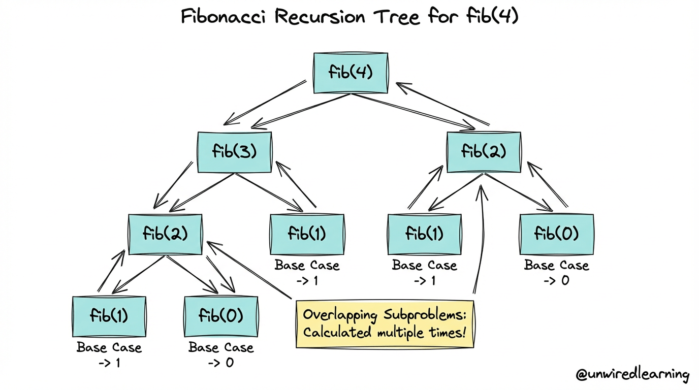
Notice the yellow box highlighting "Overlapping Subproblems." The entire sub-tree for fib(2) is computed twice! This is a critical observation that a call tree makes immediately obvious. It's a major source of inefficiency in this naive recursive solution, something we will learn to fix in a later module on Dynamic Programming.

The Order of Execution: A Depth-First Journey

A common point of confusion is the order in which the nodes in the tree are executed. JavaScript, like most languages, evaluates function arguments from left to right. In fib(n-1) + fib(n-2), the entire recursive call to fib(n-1) must complete and return its value before the call to fib(n-2) even begins.

This means the execution path follows a depth-first traversal of the call tree. It goes as deep as it can down the left-most branches first, resolves them, and then backtracks to work on the branches to the right.

This image perfectly illustrates the relationship between the call tree and the call stack at a specific moment in time.

To see this in action, let's return to the video on tree recursion, which animates the precise order of computation.

Let's Practice: Tracing a New Function

Now it's time to put this skill into practice. Let's trace the execution of the following function for an initial call of mystery(4).

function mystery(n: number): number {
  if (n < 0) {
    return 2;
  }
  return mystery(n - 1) + mystery(n - 3);
}

We will build the call tree and find the final return value. A key technique when tracing by hand is to avoid re-computing branches. Once you've figured out the result for a call like mystery(1), you can just write down that result every subsequent time you see it.

Let's summarize the trace for mystery(4) using a tree diagram.

1. mystery(4) -> calls mystery(3) + mystery(1)
2. mystery(3) -> calls mystery(2) + mystery(0)
3. mystery(2) -> calls mystery(1) + mystery(-1). Base case mystery(-1) returns 2. Now we need mystery(1).
4. mystery(1) -> calls mystery(0) + mystery(-2). Base case mystery(-2) returns 2. Now we need mystery(0).
5. mystery(0) -> calls mystery(-1) + mystery(-3). Both are base cases, returning 2. So, mystery(0) returns 2 + 2 = 4.
6. Back to mystery(1): It can now compute 4 + 2 = 6. So, mystery(1) returns 6.
7. Back to mystery(2): It can now compute 6 + 2 = 8. So, mystery(2) returns 8.
8. Back to mystery(3): It needs mystery(0). We already know mystery(0) = 4! So, mystery(3) computes 8 + 4 = 12.
9. Back to mystery(4): It needs mystery(1). We already know mystery(1) = 6! So, mystery(4) computes 12 + 6 = 18.

The final answer is 18. By drawing the tree and reusing results, we can systematically solve the problem without getting lost.

Conclusion

In this lesson, we demystified recursive execution by connecting it to the familiar concept of the call stack and introducing the call tree as a powerful visualization tool.

Here are the main takeaways:

• Recursive calls are managed by the function call stack, just like any other function call.
• A call tree is a diagram that maps out all the recursive calls made during an execution. Each node is a call, and its children are the calls it makes.
• Tree recursion occurs when a function makes more than one recursive call, leading to a branching call tree.
• The execution of a call tree happens in a depth-first order.
• Call trees are invaluable for understanding a recursive algorithm's behavior, identifying inefficiencies like overlapping subproblems, and debugging.

In our next lesson, we will use the call tree to perform our first real algorithmic analysis. We will learn how to estimate the total number of calls, the maximum recursion depth (which corresponds to the maximum memory used by the call stack), and the associated risk of a stack overflow error in JavaScript.