Mitigating Communication Overhead: Gradient Techniques

Introduction

Welcome back. In our previous lesson, we explored the algorithmic adjustments necessary for effective large-batch training, focusing on learning rate scaling and advanced optimizers like LARS and LAMB. We established that with the right optimizer, training with very large batches is not only possible but can drastically reduce training time.

This raises two critical systems-level questions:

1. What if the ideal large batch size doesn't fit into GPU memory?
2. Even if it fits, what if synchronizing the massive gradients from this large batch across many GPUs becomes the new bottleneck?

This lesson addresses these questions directly by introducing two powerful techniques for mitigating communication and memory overhead in distributed training. We will explore gradient accumulation to simulate large batches without the memory cost, and gradient compression to reduce the amount of data sent over the network. Understanding these techniques is fundamental to designing efficient, large-scale AI training systems.

Gradient Accumulation: Simulating Large Batches

The most direct answer to the memory problem is gradient accumulation (GA). Instead of processing a single, large batch of data, we process several smaller "micro-batches" sequentially and let their gradients accumulate before updating the model's weights.

The process is as follows:

1. Run the forward and backward pass for a micro-batch.
2. The gradients are calculated and stored, but the optimizer is not called. The gradients from this pass are added to the gradients from previous micro-batches.
3. Repeat steps 1-2 for a specified number of accumulation steps.
4. After processing all micro-batches, call the optimizer once to update the model weights using the summed gradients.
5. Zero out the gradients and start the next cycle.

This procedure effectively simulates a larger "global batch" whose size is micro-batch size × number of accumulation steps.

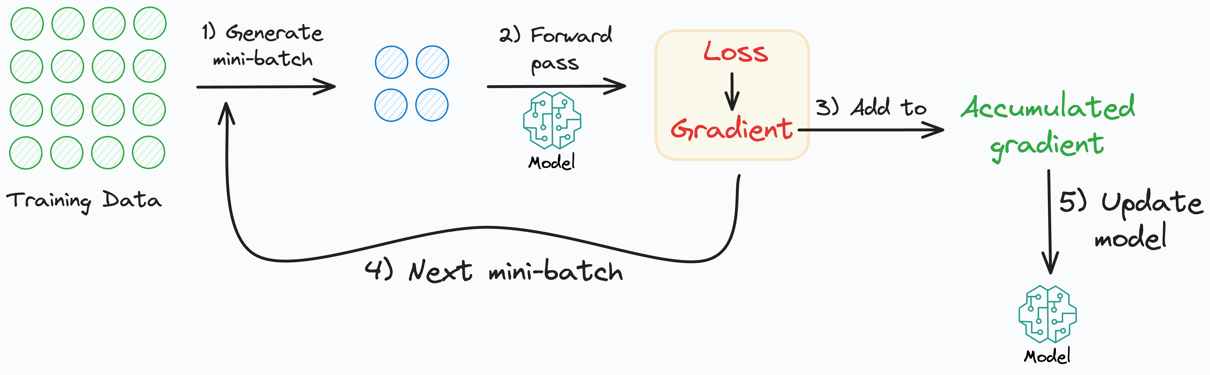
To get a deeper understanding of how this works at the level of the computation graph and its role in distributed training, the following video provides a detailed, step-by-step walkthrough.

Why and When to Use Gradient Accumulation

As the video explains, GA has two primary benefits in a distributed setting:

1. Enabling Large-Batch Training with Limited Memory: It allows you to use the large-batch optimizers we discussed in the last lesson (like LAMB) and reap their convergence benefits, even if you can't fit a batch of 32,000 into your GPU memory.
2. Reducing Communication Frequency: In synchronous data-parallel training, gradients must be synchronized across all workers using an AllReduce operation. By performing the AllReduce only once per global batch (i.e., after all accumulation steps) instead of after every micro-batch, we drastically reduce the number of communication rounds. This directly lowers the communication overhead.

Trade-offs of Gradient Accumulation

While powerful, GA is a trade-off. By processing micro-batches sequentially, we increase the total computation time for a global batch compared to processing a true large batch in parallel. You are trading more compute time for less memory usage and less frequent communication.

The following paper provides a systematic study of these trade-offs, particularly in a cloud computing context where both time and resource cost matter.

As the paper highlights, the cost-benefit analysis of GA is not always simple. In scenarios with low-bandwidth interconnects, reducing communication frequency can lead to significant savings in both time and cost, even if the per-iteration computation time increases. The paper's empirical results show that in some cases, GA can reduce total training cost by over 30% with only a moderate increase in training time.

Gradient Compression: Reducing Communication Volume

Gradient accumulation reduces communication frequency. An alternative (or complementary) approach is to reduce the communication volume at each synchronization step. This is the goal of gradient compression.

In a large model like a Transformer, the gradients can consist of hundreds of millions or billions of floating-point numbers. Transmitting all of this data for every training step can saturate the network. Gradient compression techniques aim to shrink this data before it is sent over the wire. Common methods include:

• Quantization: Reducing the numerical precision of the gradients. Instead of sending 32-bit floats (FP32), one might send 16-bit floats (FP16), 8-bit integers (INT8), or even just the 1-bit sign of the gradient (as in the SignSGD algorithm).
• Sparsification: Sending only a subset of the gradients. For example, a Top-K sparsification scheme sends only the K% of gradients with the largest magnitudes, assuming the rest are close to zero and less important for the update.
• Low-Rank Decomposition: Approximating the large gradient matrix with a product of two smaller, low-rank matrices. This is the approach used by PowerSGD.

These techniques are lossy—information is discarded. The central challenge is to compress the gradients as much as possible without harming the model's convergence.

The Utility of Compression in Modern Systems

A crucial question for a systems designer is: given the advanced optimizations in modern deep learning frameworks, is gradient compression still beneficial?

Frameworks like PyTorch DistributedDataParallel (DDP) and Horovod are highly optimized. As we will explore further in the next lesson, they use techniques to overlap communication with computation. As gradients for the last layers of a model are computed, the framework can immediately begin communicating them while the backward pass continues for the earlier layers. This "hides" much of the communication latency.

The following paper provides a rigorous analysis of this exact question.

Trade-offs and Key Findings

The paper delivers a nuanced but critical verdict for systems designers.

The Case Against Gradient Compression:

1. Encoding/Decoding Overhead: Compression is not free. The GPU must spend time encoding the gradients before sending and decoding them upon receipt. This compute overhead can sometimes be greater than the communication time saved.
2. Interference with Overlap: Gradient compression is a compute-intensive task. When you try to overlap it with the backward pass, both processes compete for the same GPU resources, potentially slowing down the entire iteration. Uncompressed communication, being a pure data transfer, can be overlapped more effectively.
3. All-Reduce Incompatibility: The highly efficient Ring-AllReduce algorithm requires an associative operation (like summation). Not all compression schemes are associative. This forces the system to fall back to a less efficient AllGather followed by local computation, which scales poorly with the number of workers.

The Case For Gradient Compression:

The paper also identifies scenarios where compression remains highly effective:

• Low-Bandwidth Environments: In clusters with slower interconnects (e.g., standard Ethernet instead of InfiniBand or NVLink), or in wide-area networks, communication is the undeniable bottleneck. Here, the savings from compression can easily outweigh the compute overhead.
• Small Batch Sizes: When using smaller batch sizes, the computation time per step is short, leaving less time to "hide" communication via overlap. In these compute-light scenarios, reducing communication volume becomes more critical.

This analysis shows that gradient compression is not a universally applicable optimization. Its utility is highly dependent on the specific hardware configuration (GPU speed, network bandwidth) and training workload (model size, batch size).

Conclusion

In this lesson, we explored two vital techniques for managing the systems-level challenges of distributed training. We've seen that optimizing large-scale ML is not just about algorithms but also about managing finite hardware resources like memory and network bandwidth.

Key Takeaways:

• Gradient Accumulation (GA) mitigates memory limitations and reduces communication frequency. It allows you to simulate very large batches by trading increased sequential computation time for lower memory pressure and fewer synchronization events.
• Gradient Compression reduces communication volume. It shrinks the size of gradient data before transmission, which is most effective in bandwidth-constrained environments.
• The utility of these techniques is a trade-off. GA costs compute time, while compression adds encoding/decoding overhead and can interfere with other optimizations.
• In modern, high-bandwidth data center environments, system-level optimizations like communication-computation overlap have significantly reduced the general-purpose utility of gradient compression, making it a more situational tool.

Preview of the Next Lesson:

We've repeatedly mentioned the importance of "communication-computation overlap." In the next lesson, we will dive deep into this concept. You will learn how frameworks use primitives like CUDA streams and asynchronous collective operations to execute data transfers and computations in parallel, effectively hiding the latency of communication and maximizing GPU utilization.