Large-Batch Training: Convergence, Scaling, and Adaptive Optimizers

Introduction

In our last lesson, we established that synchronous distributed training is algorithmically equivalent to performing standard mini-batch SGD, but with a very large "global" batch size. This approach ensures convergence stability by eliminating stale gradients. However, simply increasing the batch size is not a free lunch; it introduces a new set of complex optimization challenges.

This lesson directly addresses those challenges. We will analyze the impact of large-batch training on model convergence, a phenomenon often discussed in terms of a "generalization gap." You will learn why naive large-batch training can be detrimental and explore the two primary solutions that enable stable and effective training at scale: learning rate scaling and the development of specialized adaptive optimizers like LARS and LAMB.

The Problem with Large Batches: The "Generalization Gap"

A common empirical observation is that models trained with very large batches sometimes generalize more poorly to unseen data than models trained with smaller batches, even if they reach a similar training loss. This is often called the generalization gap.

The core intuition behind this issue relates to the geometry of the loss landscape.

• Small-batch SGD is noisy. The high variance in gradient estimates from small batches prevents the optimizer from settling into the first minimum it finds. This noise helps it escape sharp, narrow minima and find flatter, wider minima. Flatter minima are often associated with better generalization.
• Large-batch SGD has low variance. The gradient estimate is more accurate, representing the "true" gradient over a large portion of the dataset. This can cause the optimizer to aggressively descend into the nearest minimum, which may be sharp and generalize poorly.

The key takeaway from that reading is transformative: the "generalization gap" is not an inescapable fate of large batches. Instead, it stems from using a training regime (specifically, the number of updates and the learning rate schedule) designed for small batches. By adapting the training regime, the gap can be closed.

First-Line Defense: Learning Rate Scaling and Warm-up

If we use a larger batch, our gradient estimate is more reliable. It makes sense, then, that we should take a larger step in that direction. This is the motivation behind learning rate (LR) scaling.

The Linear Scaling Rule

A common heuristic is the Linear Scaling Rule: if you multiply the batch size by a factor of $k$, you should also multiply the learning rate by $k$. This rule aims to keep the expected parameter update constant per data sample, not per gradient step.

However, this aggressive scaling can cause instability, especially at the beginning of training when the model's weights are randomly initialized and far from a good solution. A very large learning rate can cause the parameters to "explode."

Learning Rate Warm-up

To counteract this instability, a learning rate warm-up strategy is used. Training begins with a small initial learning rate, which is then gradually increased over a number of "warm-up" steps until it reaches the target value determined by the scaling rule. This gives the model a chance to settle into a more stable region of the loss landscape before large steps are taken.

The Square-Root Scaling Rule

An alternative, theoretically-grounded approach is the Square-Root Scaling Rule. This rule suggests that to keep the variance of the weight updates constant, the learning rate should be scaled by $\sqrt{k}$ when the batch size is scaled by $k$.

In practice, the linear scaling rule combined with a warm-up period has been used successfully for many vision models. However, for more complex models like Transformers and at extremely large batch sizes, even these strategies reach their limits.

The Need for Adaptive Optimizers

The fundamental limitation of LR scaling is that it applies a single, uniform learning rate across all layers and parameters of the network. In reality, different layers of a deep neural network learn at different rates. The gradients for embedding layers might be sparse and have a different magnitude compared to the final classification layer. A single learning rate cannot be optimal for all of them.

This issue is exacerbated in large-batch training. The aggressive learning rate required for some layers might be destructively large for others. This led to the development of optimizers that adapt the learning rate on a per-layer basis.

Advanced Solution: LARS and LAMB Optimizers

The key innovation to unlock massive batch sizes was to create optimizers that adapt the update magnitude for each layer independently.

Let's study the paper that introduced the LAMB optimizer, which builds directly on its predecessor, LARS.

Let's break down the core ideas from that paper.

LARS: Layer-wise Adaptive Rate Scaling

The LARS algorithm implements a simple but powerful idea. For each layer $i$, it computes a unique learning rate based on a "trust ratio." The update rule for a layer $i$ looks like this:

Where:

• $w^{(i)}$ are the weights of layer $i$.
• $m^{(i)}$ is the momentum-updated gradient for layer $i$.
• ${\eta }_t$ is the global learning rate.
• $\varphi (\Vert w_t^{(i)}\Vert )$ is a function of the norm of the layer's weights (often just $\Vert w_t^{(i)}\Vert$).

The core of LARS is the trust ratio: $\frac{\Vert w_t^{(i)}\Vert }{\Vert m_t^{(i)}\Vert }$. It scales the update size. If the gradient norm is large relative to the weight norm, the trust ratio is small, preventing a large, potentially unstable update. If the gradient norm is small, the update is scaled up. This adaptively normalizes the update magnitude for each layer, preventing any single layer's gradients from dominating the learning process.

LAMB: Layer-wise Adaptive Moments for Batching

LAMB extends LARS by incorporating the element-wise adaptive machinery of the Adam optimizer. Adam maintains moving averages of the first moment (the mean, $m_t$) and the second moment (the uncentered variance, $v_t$) of the gradients for each parameter. It uses these to compute a parameter-specific update.

LAMB computes the Adam update step, but then applies the LARS-style layer-wise normalization to it.

Looking at Algorithm 2 in the paper, you can see the process:

1. Compute $m_t$ and $v_t$ just like in Adam.
2. Compute an update ratio $r_t=m_t/(\sqrt{v_t}+ϵ)$. This is the Adam part, normalizing each gradient component by its historical magnitude.
3. Apply a LARS-style normalization to this ratio at the layer level: $$w_{t+1}^{(i)}=w_t^{(i)}-{\eta }_t\cdot \frac{\varphi (\Vert w_t^{(i)}\Vert )}{\Vert r_t^{(i)}\Vert }\cdot r_t^{(i)}$$

LAMB effectively gets the best of both worlds: Adam's per-parameter adaptivity and LARS's layer-wise stability for large-batch training. This combination proved exceptionally powerful for training large Transformer models like BERT.

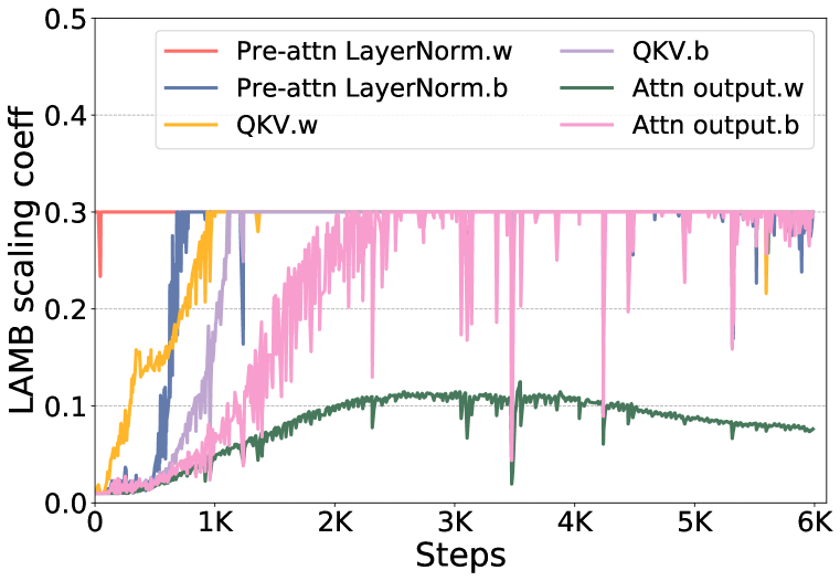
The results speak for themselves. The authors of the LAMB paper used it to scale BERT training to a batch size of over 32,000, reducing the training time from 3 days to just 76 minutes.

The Role of the Optimizer: Direction vs. Magnitude

It's helpful to think of an optimizer's job as having two components: choosing the direction of the update and choosing the magnitude (step size) of the update.

• The gradient itself provides the direction.
• The learning rate schedule and optimizer mechanics determine the magnitude.

What LARS, LAMB, and other research show is that for large-batch training, accurately controlling the magnitude of the update, especially on a per-layer basis, is often more critical than refining the direction.

This perspective helps clarify why LARS and LAMB are so effective. They are meticulously engineered to control the update magnitude at the layer-level, providing the stability needed to use the very large learning rates that large-batch training demands.

Conclusion

In this lesson, we dissected the challenges of large-batch training and the sophisticated solutions developed to overcome them. We moved from a simple problem statement to the state-of-the-art optimizers that power today's largest models.

Key Takeaways:

• Large-batch training can suffer from a generalization gap, where models converge to sharp minima that generalize poorly.
• This gap is not fundamental to the batch size but to the training regime. It can be closed by adapting the number of training iterations and optimizer settings.
• A first-level solution involves using a learning rate scaling rule (linear or square-root) in conjunction with a learning rate warm-up period to maintain stability.
• The most robust solution involves layer-wise adaptive optimizers. LARS introduces a layer-specific "trust ratio" to normalize updates, while LAMB combines this with Adam's per-parameter moment tracking, making it highly effective for complex models.

Preview of the Next Lesson:

We have now addressed the algorithmic consequences of using large batches. However, using a massive batch size isn't always feasible due to GPU memory constraints. In our next lesson, we will explore techniques for mitigating communication overhead and managing memory, such as gradient accumulation, which allows us to achieve the benefits of a large batch size without needing to fit it all in memory at once, and gradient compression, which reduces the amount of data that needs to be synchronized.