DFS: Recursive & Iterative Implementations

What is Depth-First Search?

Depth-First Search is an algorithm for traversing a graph. As the name suggests, it prioritizes depth. Imagine you're exploring a maze. DFS is like choosing one path and following it as far as you can go. When you hit a dead end, you backtrack to the last junction where you had an unexplored path, and you dive down that new path. You repeat this until all paths from your starting point have been explored.

This "dive deep, then backtrack" strategy is a powerful tool for many problems, including finding paths, detecting cycles, and exploring all possible solutions in a search space.

To get a feel for this process, take a look at the following image which illustrates a step-by-step DFS traversal on a tree.

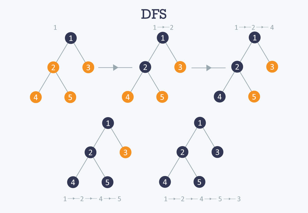
A crucial element in any graph traversal is keeping track of where you've already been. Without this, if the graph contains a cycle (e.g., A -> B -> C -> A), the algorithm would loop forever. To prevent this, we use a set (often called visited or seen) to store the nodes we have already processed.

For a more dynamic and intuitive explanation of this core idea, the following video is highly recommended.

Recursive Implementation of DFS

The "dive deep and backtrack" nature of DFS maps perfectly to recursion. The act of "diving deep" is simply a recursive call on a neighbor. When that call finishes, the function returns, which is the "backtracking" step. The program's own call stack implicitly manages the path for us.

The logic is straightforward:

1. Start at a given node. Mark it as visited.
2. Process the node (e.g., print its value).
3. For each neighbor of the current node:
4. If the neighbor has not been visited, recursively call the DFS function on it.

Let's see this translated into Python code. The following video implements this logic using the defaultdict adjacency list we created in the last lesson.

Here is the code, which you should be able to follow along with the video:

from collections import defaultdict

# Assume 'adj' is our adjacency list (a defaultdict)
# adj = defaultdict(list)
# ... edges are added here ...

# Set to keep track of visited nodes
seen = set()

def dfs_recursive(graph, node):
    # Process the node (e.g., print it)
    print(node, end=" ")
    
    # Mark the current node as seen
    seen.add(node)
    
    # Recurse for all adjacent vertices that haven't been seen
    for neighbor in graph[node]:
        if neighbor not in seen:
            dfs_recursive(graph, neighbor)

# --- Example Usage ---
# Build the graph from the video
edges = [[0, 1], [0, 3], [1, 2], [3, 4], [3, 6], [3, 7], [4, 5], [4, 2], [5, 2], [5, 4]]
n = 8
adj = defaultdict(list)
for u, v in edges:
    adj[u].append(v)

print("Recursive DFS traversal:")
# To start the traversal, call the function with the starting node
start_node = 0
dfs_recursive(adj, start_node)
print("\n")

The recursive approach is often preferred for its simplicity and readability when the graph isn't excessively deep.

Iterative Implementation of DFS

While recursion is elegant, it has a limitation: Python has a recursion depth limit. For very deep graphs (like a long linked list), a recursive DFS could cause a RecursionError. The solution is an iterative implementation using an explicit stack.

The logic is as follows:

1. Create a stack and push the start_node onto it.
2. Create a seen set to track visited nodes.
3. While the stack is not empty:
4. Pop a node from the stack.
5. If the node has already been seen, continue.
6. Mark the node as seen and process it.
7. Push all unseen neighbors of the node onto the stack.

The following video clip demonstrates this iterative approach.

Here is the corresponding Python code:

def dfs_iterative(graph, start_node):
    seen = set()
    stack = [start_node] # Start with the initial node
    
    while stack:
        node = stack.pop() # Get the last node added
        
        if node not in seen:
            # Process the node
            print(node, end=" ")
            seen.add(node)
            
            # Add all unseen neighbors to the stack.
            # Note: The order of traversal can depend on the order neighbors are added.
            # To match the typical recursive order, you might add them in reverse.
            for neighbor in reversed(graph[node]): # reversed() is optional but can help consistency
                if neighbor not in seen:
                    stack.append(neighbor)

# --- Example Usage ---
# Using the same adjacency list 'adj' from before
print("Iterative DFS traversal:")
dfs_iterative(adj, start_node=0)
print("\n")

Notice the traversal order might differ from the recursive one. This is because the recursive version explores the first neighbor deeply, while the iterative version adds all neighbors to the stack and then explores the last one added. This difference is generally fine unless a specific traversal order is required by a problem.

graph = {
    0: [1, 2],
    1: [0, 3],
    2: [0, 3],
    3: [1, 2, 4],
    4: [3]
}

Complexity and When to Use Which

For a graph with $V$ vertices and $E$ edges, both implementations of DFS have the same complexity:

• Time Complexity: $O(V+E)$. This is because in the worst case, DFS visits every vertex and traverses every edge exactly once.
• Space Complexity: $O(V)$. In the recursive version, this space is used by the call stack (which can be as deep as the number of vertices in the worst case, e.g., a path graph). In the iterative version, this is the space used by the stack and the seen set.

Recursive vs. Iterative:

• Recursive: Simpler to write and read. Excellent for most competitive programming scenarios.
• Iterative: Use this if you anticipate a very deep graph that might cause a stack overflow, or if you need finer control over the stack's contents.

Conclusion

You have now mastered Depth-First Search, a cornerstone of graph algorithms. You understand its core principle and can confidently implement it both recursively and iteratively.

Key Takeaways:

• DFS explores a graph by going as deep as possible down one path before backtracking.
• A seen set is essential to track visited nodes and prevent infinite loops in graphs with cycles.
• The recursive implementation is elegant and uses the system's call stack to manage backtracking. Its time complexity is $O(V+E)$.
• The iterative implementation uses an explicit stack (e.g., a Python list) to avoid recursion limits, making it more robust for very deep graphs. It shares the same $O(V+E)$ time complexity.

Up Next:
In the next lesson, we will explore the other fundamental graph traversal algorithm: Breadth-First Search (BFS). You'll see how a simple switch from a stack to a queue completely changes the traversal strategy from "depth-first" to "level-by-level", and you'll learn which types of problems are best suited for each.