DSU for Connectivity: Provinces Problem

1. Understanding the "Provinces" Problem

Imagine a map with several cities, where some cities are connected by roads. A "province" is a group of cities where you can travel from any city in the group to any other city in the same group, but you cannot travel to a city in a different province. The task is to count how many such separate provinces exist.

In graph theory terms, a province is a connected component.

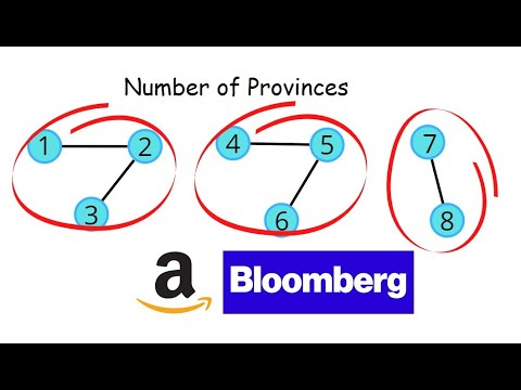
While you could solve this using graph traversal algorithms like Depth-First Search (DFS) or Breadth-First Search (BFS), DSU offers a more direct and often more efficient approach, especially for dynamic connectivity scenarios.

2. The DSU Strategy for Counting Components

The core idea is to model the problem using disjoint sets. Here's how we map the graph problem to our DSU data structure:

1. Initialization: We start by assuming each of the n nodes (cities) is its own isolated province. So, we initialize our DSU with n elements, and our initial province count is n.
2. Processing Edges: We iterate through all the connections (edges) in the graph. For each edge connecting nodes u and v, we perform a union(u, v) operation.
3. Merging Provinces: The union operation attempts to merge the sets containing u and v.
   • If u and v were in different sets (provinces), the union operation succeeds, and we have effectively merged two provinces into one. Therefore, we decrement our province count by 1.
   • If u and v were already in the same set, the union operation does nothing because they are already connected. The province count remains unchanged.
4. Final Count: After processing all the edges, the final value of our province counter is the answer.

This approach elegantly uses the boolean return value from the union method we designed in the last lesson to track the number of components dynamically.

3. A Step-by-Step Walkthrough

Let's watch a video that implements this exact logic to solve the "Number of Connected Components" problem. The problem is identical to finding the number of provinces.

4. The Python Implementation

As you saw in the video, the implementation is surprisingly concise once you have your UnionFind class. Let's assume you have the UnionFind class we built in the previous lesson. The function to count components would look like this:

# Assume this class is defined from the previous lesson
class UnionFind:
    def __init__(self, n):
        self.parent = list(range(n))
        self.rank = [1] * n
    
    def find(self, x):
        if self.parent[x] != x:
            self.parent[x] = self.find(self.parent[x]) # Path compression
        return self.parent[x]

    def union(self, x, y):
        root_x = self.find(x)
        root_y = self.find(y)
        
        if root_x != root_y:
            # Union by rank logic
            if self.rank[root_x] > self.rank[root_y]:
                self.parent[root_y] = root_x
            elif self.rank[root_x] < self.rank[root_y]:
                self.parent[root_x] = root_y
            else:
                self.parent[root_y] = root_x
                self.rank[root_x] += 1
            return True # Important: indicates a successful merge
        return False # Indicates they were already connected

# The solution function
def count_provinces(n, edges):
    """
    Counts the number of connected components in a graph.
    
    Args:
        n (int): The number of nodes (from 0 to n-1).
        edges (list of lists): A list of edges, e.g., [[0, 1], [1, 2]].
    """
    if n == 0:
        return 0
        
    uf = UnionFind(n)
    num_components = n # Start with n components
    
    for u, v in edges:
        # If union is successful, it means we merged two previously
        # separate components.
        if uf.union(u, v):
            num_components -= 1
            
    return num_components

# Example usage:
nodes = 5
connections = [[0, 1], [1, 2], [3, 4]]
print(f"Number of provinces: {count_provinces(nodes, connections)}") # Output: 2

This code directly implements the strategy we discussed. It initializes the count to n and decrements it every time the union function confirms that two separate components have been merged.

5. An Alternative Counting Method

There's another common way to count the components, which is conceptually simple but might be slightly less efficient as it requires a final loop. Instead of decrementing a counter, you can wait until all union operations are done and then count the number of unique roots.

This line of code does the following:

1. It iterates through every node x from 0 to n-1.
2. For each node, it calls uf.find(x) to get the root of its component.
3. It adds all these roots to a set, which automatically handles duplicates.
4. The final number of components is simply the size (len) of the set of unique roots.

Both methods are correct and widely used. The decrementing-counter method is slightly more performant as it avoids the final loop, but the unique-root-counting method is also perfectly acceptable and easy to remember.

Conclusion

You have successfully applied your DSU data structure to a practical graph problem. This pattern of initializing n components and merging them based on edge connections is fundamental to solving many connectivity-based problems in competitive programming.

Key Takeaways:

• A connected component (or "province") in a graph can be modeled as a set in the DSU data structure.
• The strategy is to initialize n components and process each edge with a union operation.
• You can count components by either:
  1. Decrementing a counter each time a union operation successfully merges two components.
  2. Counting the number of unique roots after all union operations are complete.
• DSU provides an elegant and efficient solution for this type of problem.

Up Next:
In the next lesson, we will continue exploring the power of DSU by tackling another critical application: implementing Kruskal's algorithm to find a Minimum Spanning Tree (MST). You'll see how DSU's ability to efficiently detect if two nodes are already connected is the key to building the MST.