Counting Sort for Limited-Range Integers

What is Counting Sort and Why Use It?

All the sorting algorithms we've discussed so far—Merge Sort, Quicksort, and Python's built-in sort—are comparison-based. They work by comparing pairs of elements to decide their order. It's a proven fact in computer science that any comparison-based sorting algorithm has a lower bound of $O(n\log n)$ time complexity in the average and worst case.

Counting Sort breaks this barrier. It doesn't compare elements at all. Instead, it works by counting the number of occurrences of each unique element in the input array. This allows it to sort in linear time, but it comes with a major condition: it's only efficient for sorting integers that fall within a limited range.

For a great animated introduction to why Counting Sort is useful and the scenarios where it excels, watch the beginning of the following video.

How Counting Sort Works: A Step-by-Step Guide

The core idea is simple: if we know how many elements are less than a given element x, we can place x directly into its correct sorted position.

Let's break down the algorithm into two main versions: a simple, intuitive approach and a more robust, stable version. A stable sorting algorithm maintains the relative order of equal elements, which can be important in some problems.

Version 1: The Simple (In-place) Approach

This version is easy to understand and implement. It involves two main passes over the data.

1. Count Frequencies: Create a count array to store the frequency of each number in the input array. To do this, you first need to find the maximum value in the input array to determine the size of the count array.
2. Reconstruct the Array: Iterate through the count array from the smallest index to the largest. For each number i, append i to the result count[i] times. This overwrites the original array with the sorted elements.

This approach is demonstrated very clearly in the following video, which is geared towards competitive programming.

While this method works for sorting simple integers, it is not stable. For example, if you were sorting objects based on an integer key, you wouldn't be able to preserve their original relative order if they had the same key. That's where the stable version comes in.

Version 2: The Stable Approach

This version is slightly more complex but is the standard, more powerful implementation. It ensures stability.

1. Find the maximum value (max_val) in the input array.
2. Create a count array of size max_val + 1 and store the frequency of each element, just like before.
3. Calculate cumulative counts: Modify the count array so that each element at index i stores the sum of counts up to i. After this step, count[i] tells you the position where the last occurrence of element i should go in the sorted output.
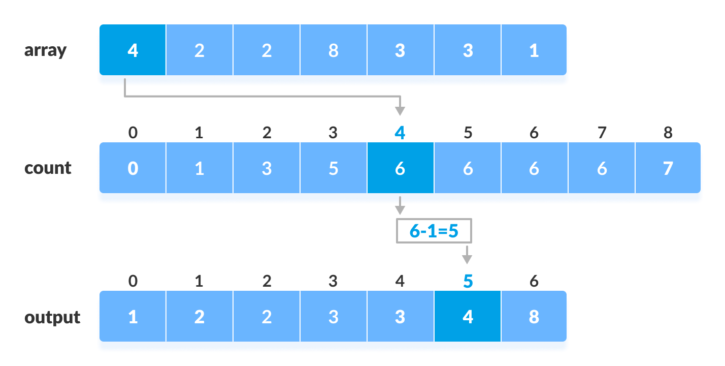
4. Build the output array: Create a new output array of the same size as the input. Iterate through the input array in reverse. For each element x, place it at output[count[x] - 1], and then decrement count[x]. Iterating in reverse is the key to maintaining stability.

The Programiz article below provides excellent diagrams illustrating this process.

This image from the article perfectly captures the final step of placing an element into the output array using the cumulative counts.

Python Implementation

Now, let's translate the stable algorithm into Python code. The following implementation is clear and directly follows the steps we just outlined.

Here's the code from the article for your reference:

def counting_sort(arr):
    # Step 1: Find the maximum value in the array
    max_val = max(arr)

    # Step 2: Create a count array of size (max_val + 1) initialized to zero
    count = [0] * (max_val + 1)

    # Step 3: Count occurrences of each element
    for num in arr:
        count[num] += 1

    # Step 4: Transform count array to store actual positions (cumulative sum)
    for i in range(1, len(count)):
        count[i] += count[i - 1]

    # Step 5: Build the sorted output array
    output = [0] * len(arr)
    # Iterate in reverse for stability
    for num in reversed(arr):
        output[count[num] - 1] = num
        count[num] -= 1
        
    return output

# Example usage
arr = [4, 2, 2, 8, 3, 3, 1]
sorted_arr = counting_sort(arr)
print("Sorted array:", sorted_arr)
# Output: Sorted array: [1, 2, 2, 3, 3, 4, 8]

Complexity Analysis and Trade-offs

Understanding the performance of Counting Sort is key to knowing when to use it in a competition.

• Time Complexity: $O(n+k)$, where $n$ is the number of elements in the input array, and $k$ is the range of the input values (specifically, max_val).
  • Finding the max: $O(n)$
  • Counting frequencies: $O(n)$
  • Calculating cumulative sums: $O(k)$
  • Building the output array: $O(n)$
  • Total: $O(n+n+k+n)=O(3n+k)$, which simplifies to $O(n+k)$.
• Space Complexity: $O(n+k)$. We need $O(k)$ for the count array and $O(n)$ for the output array.

This complexity analysis reveals the algorithm's main strength and weakness. If $k$ is small or on the same order as $n$ (i.e., $k\approx n$), the time complexity is effectively $O(n)$, which is fantastically fast. However, if you have an array like [1, 10000000], then $k$ would be enormous, making the algorithm incredibly slow and memory-hungry. This makes it unsuitable for sorting data with a large range of values.

Conclusion

Great work today! You've added a non-comparison-based sorting algorithm to your toolkit. Counting Sort is a prime example of how understanding the properties of your data can lead to significant performance gains, a crucial insight for competitive programming.

Key Takeaways:

• Counting Sort is a non-comparison sorting algorithm that achieves linear time complexity, $O(n+k)$.
• It is only effective for sorting integers within a limited range (k).
• It works by counting element frequencies and using those counts to determine the final sorted positions.
• The stable version uses a cumulative count array and is generally preferred.
• Its primary weakness is high time and space complexity when the range of numbers (k) is very large compared to the number of elements (n).

Up Next:
Now that you have a solid foundation in various sorting algorithms, we'll move on to a new class of techniques that often operate on sorted data. In our next lesson, we'll dive into the Two-Pointers and Sliding Window module, starting with how to "Apply the two-pointer technique to solve problems on sorted arrays." You'll see how a sorted array can be processed very efficiently using this clever pattern.