Custom Plot: Axes and Labels

The Goal: From Canvas to Plot

Our objective is to transform our blank canvas into a structured plot with clear visual guides.

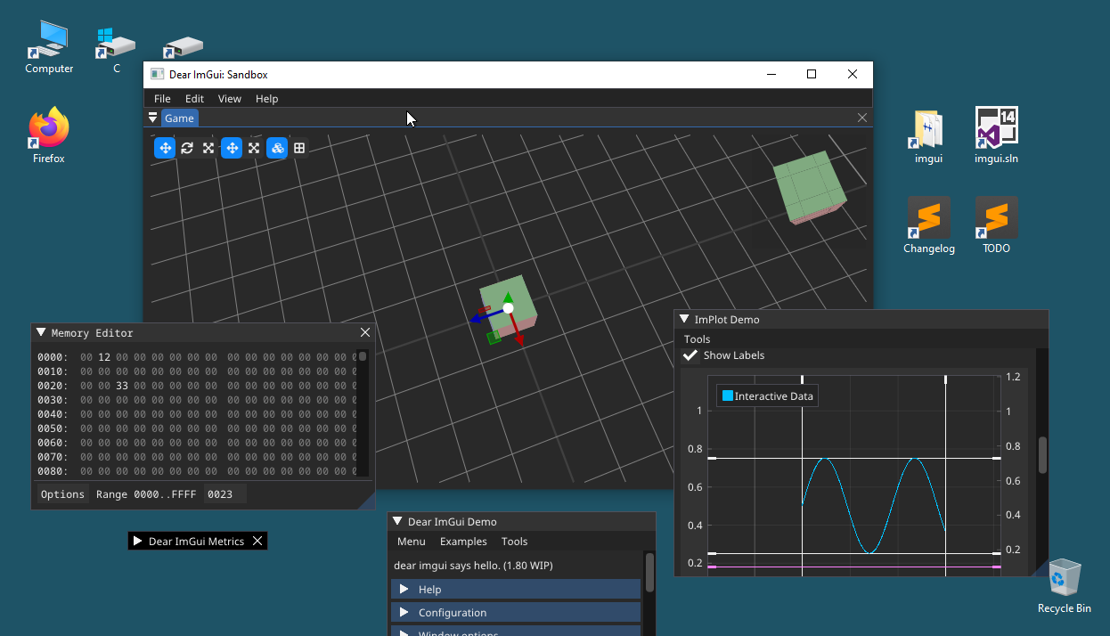
ImGui's built-in PlotLines function is too basic for this, and creating a custom plot like ours means we have to draw these elements ourselves. As the author of ImGui himself notes, this is a common need that is best met by using the ImDrawList API to create your own customized graph.

The Anatomy of an Axis

Let's break down what we need to draw. A complete axis consists of several parts:

• Grid Lines: A set of horizontal and vertical lines at regular intervals that provide a background reference.
• Tick Marks: Small lines perpendicular to the axis line that mark specific values.
• Tick Labels: The numbers or text corresponding to the tick marks.

For today, we will focus on drawing the grid lines and their corresponding labels. We'll draw them across the entire plot area.

Drawing the Grid

The core idea is simple: grid lines are just a series of lines drawn at fixed intervals in world space. Because their positions are defined in the same coordinate system as our data, our existing WorldToScreen function will automatically handle positioning them correctly as you pan and zoom.

Here is the algorithm:

1. Define a Grid Step: Choose an interval in world units for your grid lines (e.g., every 100.0 units).
2. Find the Visible World Range: Use your ScreenToWorld function on the corners of your canvas to find the minimum and maximum visible X and Y coordinates.
3. Find the First Grid Line: Calculate the first grid line that is visible. For example, if your visible X-range starts at 435.0 and your step is 100.0, the first visible line is at 500.0. A little bit of integer math helps here: startX = floor(visible_min_x / grid_step) * grid_step;
4. Loop and Draw: Loop from that starting point until you pass the maximum visible coordinate, incrementing by grid_step each time. In each iteration:
   • Convert the world-space position of the line into screen-space using WorldToScreen.
   • Use draw_list->AddLine() to draw it.

Let's add this to our PlotMyData function. This code should go after the pan/zoom input handling but before you draw your data series.

// ... inside PlotMyData, after input handling ...
ImDrawList* draw_list = ImGui::GetWindowDrawList();

// Define colors
const ImU32 grid_color = IM_COL32(200, 200, 200, 40);
const ImU32 text_color = IM_COL32(255, 255, 255, 200);

// --- Draw Grid and Labels ---

// 1. Define grid step in world units
const float grid_step_x = 100.0f;
const float grid_step_y = 0.5f;

// 2. Find visible world range
ImVec2 world_p0 = ScreenToWorld(canvas_p0, pan_offset, zoom_level, canvas_p0, canvas_p1);
ImVec2 world_p1 = ScreenToWorld(canvas_p1, pan_offset, zoom_level, canvas_p0, canvas_p1);

// 3. Draw vertical grid lines and X-axis labels
for (float x = std::floor(world_p0.x / grid_step_x) * grid_step_x; x < world_p1.x; x += grid_step_x) {
    // Convert world x to screen x
    ImVec2 screen_pos = WorldToScreen(ImVec2(x, 0), pan_offset, zoom_level, canvas_p0, canvas_p1);

    // Check if the line is within the canvas bounds before drawing
    if (screen_pos.x >= canvas_p0.x && screen_pos.x <= canvas_p1.x) {
        // Draw the grid line
        draw_list->AddLine(ImVec2(screen_pos.x, canvas_p0.y), ImVec2(screen_pos.x, canvas_p1.y), grid_color);
        
        // Draw the label text
        char label_buf[16];
        snprintf(label_buf, sizeof(label_buf), "%.0f", x);
        draw_list->AddText(ImVec2(screen_pos.x + 2, canvas_p1.y - 15), text_color, label_buf);
    }
}

// TODO: Draw horizontal grid lines and Y-axis labels

// ... then draw the data series ...

A few notes on the code:

• We use std::floor to snap our starting grid line to a multiple of grid_step_x.
• snprintf is a C-style function that formats a number into a character buffer. It's a simple and performant way to create our labels.
• We draw the text slightly offset from the grid line (+2 pixels) and near the bottom of the canvas (canvas_p1.y - 15) for readability.

// 4. Draw horizontal grid lines and Y-axis labels
for (float y = std::floor(world_p1.y / grid_step_y) * grid_step_y; y > world_p0.y; y -= grid_step_y) {
    // Convert world y to screen y
    ImVec2 screen_pos = WorldToScreen(ImVec2(0, y), pan_offset, zoom_level, canvas_p0, canvas_p1);

    // Check if the line is within the canvas bounds before drawing
    if (screen_pos.y >= canvas_p0.y && screen_pos.y <= canvas_p1.y) {
        // Draw the grid line
        draw_list->AddLine(ImVec2(canvas_p0.x, screen_pos.y), ImVec2(canvas_p1.x, screen_pos.y), grid_color);

        // Draw the label text
        char label_buf[16];
        snprintf(label_buf, sizeof(label_buf), "%.2f", y);
        // Position the label on the left side of the canvas
        draw_list->AddText(ImVec2(canvas_p0.x + 2, screen_pos.y + 2), text_color, label_buf);
    }
}

Learning from Professional APIs

We have now implemented the basic mechanics of drawing axes. As you can imagine, a full-featured plotting library would offer many more options for styling and configuration. We can look at the API of a library like ImPlot to see how these concepts are structured professionally. We won't be using this library, but studying its design is a valuable exercise.

This exploration should give you a sense of direction. Our manual implementation is the first step, and by understanding how it's built, you gain a deeper appreciation for the abstractions that such libraries provide.

A Known Limitation: The "Wall of Lines"

Try running your code now. Pan and zoom around. It works! But if you zoom out far enough, you'll notice a problem: the grid lines and labels become so dense that they form a solid block, making the plot unreadable.

This happens because our grid_step is fixed. A step of 100.0 is reasonable when you're looking at a range of a few thousand units, but it's far too small when you're looking at a range of millions.

The solution, which we will tackle in later lessons, is Level of Detail (LOD). A robust plotter must dynamically adjust the grid step based on the zoom level, showing coarse grid lines when zoomed out and progressively finer ones as you zoom in. This is a core concept that we will revisit when we build the LOD Plotter for our data as well.

Conclusion

Congratulations! You have successfully added a crucial layer of context to your plotter. It now provides the visual reference frame needed for meaningful data analysis.

Key Takeaways:

• Custom plots in ImGui require manual rendering of axes and labels using the ImDrawList API.
• Grid lines and labels should be defined in world space so they pan and zoom correctly with the data.
• The process involves looping through visible world coordinates at a fixed step, converting each coordinate to screen space, and drawing lines (AddLine) and text (AddText).
• A "basic" implementation has limitations, such as a fixed grid density, which highlights the need for more advanced Level-of-Detail techniques that we will explore later.

What's Next?

Our plot is now navigable and understandable. The final piece of fundamental interactivity is to query the data itself. In the next lesson, you will learn to handle user input from the mouse (position, clicks) for interactivity. Specifically, we will implement a feature to display a tooltip with the precise data value when the user hovers their mouse over the plot.