Advanced Window Functions: Ranking and Offsetting

The "Window": A New Way to Look at Your Data

Before we dive into specific functions, we need to understand the core concept. A window function performs a calculation for each row, using a "window" of related rows. The key is that this calculation is added as a new column to your result set, without changing the number of rows.

The OVER() clause is what defines this window. It has two main components:

• PARTITION BY: This divides the rows into groups, or "partitions." The window function is then applied independently to each partition. It's like GROUP BY, but it doesn't collapse the rows. If you omit this, the entire result set is treated as a single partition.
• ORDER BY: This specifies the order of rows within each partition. This is crucial for ranking and for functions that depend on sequence, like LAG and LEAD.

The following video from techTFQ provides an excellent introduction to this concept, contrasting it with the familiar GROUP BY and explaining the OVER(PARTITION BY ...) syntax.

Ranking Rows: ROW_NUMBER, RANK, and DENSE_RANK

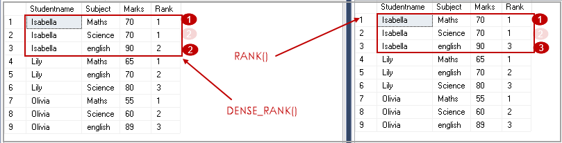
A common analytical task is to rank items within a group—for example, ranking employees by salary within each department or ranking products by sales within each category. SQL provides three primary functions for this, and the difference between them lies in how they handle ties (i.e., identical values in the ordering column).

• ROW_NUMBER(): Assigns a unique, sequential number to each row within the partition. It arbitrarily breaks ties.
• RANK(): Assigns the same rank to rows with tied values. However, it then skips the next rank(s). For example, if two rows are tied for 2nd place, they both get rank 2, and the next rank assigned is 4.
• DENSE_RANK(): Assigns the same rank to tied rows but does not skip any ranks. If two rows are tied for 2nd, they both get rank 2, and the next rank is 3.

This article provides a concise explanation with a clear table and example.

To visualize this crucial difference, consider this comparison:

Filtering on a Rank: A Job for CTEs

A very common pattern is to find the "Top N" items per group, such as the "top 3 selling products in each category." Your first instinct might be to write WHERE rank <= 3, but this will fail. Window functions are processed after the WHERE clause, so you cannot filter on their results directly.

This is where your knowledge of CTEs from the previous lesson becomes essential. The correct pattern is to first calculate the rank within a CTE, and then filter on that rank in the outer query.

Looking Forwards and Backwards: LAG and LEAD

Another powerful capability of window functions is accessing data from other rows within the same result set. This is invaluable for time-series analysis, like calculating month-over-month growth or finding the time between events.

• LAG(column, offset, default_value): "Looks back" a specified number of rows (offset, default is 1) and returns the value of the column from that row.
• LEAD(column, offset, default_value): "Looks forward" a specified number of rows and returns the value of the column from that row.

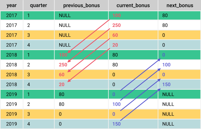
The video below gives an excellent, practical demonstration of calculating month-over-month sales changes—a classic business intelligence task.

Your Turn: Hands-On with Metabase

Let's apply these concepts to answer some analytical questions using the Metabase sample database.

Question 1: "Who are the top 3 customers in terms of total money spent?"

This is a simple ranking problem. We first need to calculate the total amount spent by each customer and then rank them.

1. Navigate to the SQL editor in Metabase.
2. Run the following query:

WITH customer_totals AS (
  SELECT
    user_id,
    SUM(total) AS total_spent
  FROM orders
  GROUP BY user_id
)
SELECT
  user_id,
  total_spent,
  DENSE_RANK() OVER (ORDER BY total_spent DESC) AS customer_rank
FROM customer_totals
ORDER BY customer_rank;

Here, we use DENSE_RANK() because if two customers spent the exact same amount, we'd want to give them the same rank without skipping the next one. We wrap the initial aggregation in a CTE for clarity.

Question 2: "For each product, what was the date of the previous order?"

This is a classic use case for LAG(). We want to look back at the previous row for a given product.

1. Run this query in the SQL editor:

SELECT
  p.title AS product_title,
  o.created_at AS order_date,
  LAG(o.created_at, 1) OVER (PARTITION BY o.product_id ORDER BY o.created_at) AS previous_order_date
FROM orders AS o
JOIN products AS p ON o.product_id = p.id
ORDER BY p.title, o.created_at;

Let's break this down:

• PARTITION BY o.product_id: This is critical. It ensures that LAG() only looks at orders for the same product. The calculation restarts for each new product ID.
• ORDER BY o.created_at: This sorts the orders chronologically within each product's partition, ensuring "previous" means the one that happened right before.
• LAG(o.created_at, 1): This looks back one row in the ordered partition to fetch the created_at value.

You'll see that for the very first order of any product, the previous_order_date is NULL, which is correct.

Conclusion

In this lesson, you've added some of the most powerful tools in analytical SQL to your toolkit. You can now perform calculations that relate one row to many others without losing the context of the individual row. This is a fundamental shift from the simple aggregation you've used before.

Key Takeaways:

• Window vs. GROUP BY: Window functions calculate values over a set of rows but return a value for each row, whereas GROUP BY collapses rows into a single summary.
• The OVER() Clause: This is the heart of window functions. PARTITION BY defines the groups, and ORDER BY defines the sequence within those groups.
• Ranking Functions: ROW_NUMBER(), RANK(), and DENSE_RANK() are used to order rows, with key differences in how they handle ties.
• Offset Functions: LAG() and LEAD() allow you to access data from preceding or succeeding rows, which is essential for trend and time-series analysis.
• CTEs are Essential: To filter on the results of a window function, you must first compute the function within a CTE or subquery.

You've learned how to rank results and compare rows to their neighbors. In our next lesson, we will continue our exploration of window functions by learning how to calculate running totals and moving averages. This will introduce another facet of the OVER() clause—the frame clause—allowing you to define an even more specific and dynamic "window" for your calculations.