Window Functions for Running Totals and Moving Averages

Running Totals: Accumulating Value Over Time

In the previous lesson, the window was defined by PARTITION BY and ORDER BY. When using aggregate functions, this structure gets an additional, often implicit, component: the frame. Let's start with a running total, also known as a cumulative sum. This is the sum of a value from the beginning of a partition up to the current row.

A common business question is, "How has our total revenue accumulated over time?" You can answer this by using SUM() as a window function.

You might be wondering why just adding ORDER BY creates a running total. The reason is that SQL applies a default window frame. When ORDER BY is present, the default frame is ROWS BETWEEN UNBOUNDED PRECEDING AND CURRENT ROW. This means for each row, the function aggregates all values from the very first row of the partition up to the current one.

The following video from Data with Baraa clearly explains this default behavior.

While the default behavior is convenient, it is a best practice to be explicit about your window frame for clarity and to avoid unexpected behavior. We'll explore the syntax for this next.

Defining the Window Frame

The window frame clause gives you precise control over the set of rows used in the calculation relative to the current row. This is where you unlock the full power of aggregate window functions.

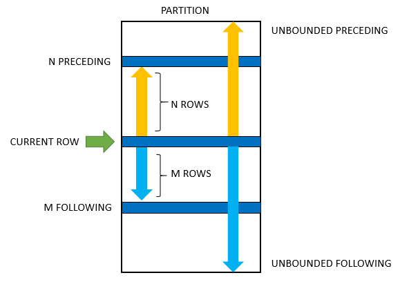
The basic syntax is ROWS BETWEEN <start> AND <end>, where <start> and <end> can be:

• UNBOUNDED PRECEDING: The first row of the partition.
• N PRECEDING: A specific number of rows before the current row.
• CURRENT ROW: The row being processed.
• N FOLLOWING: A specific number of rows after the current row.
• UNBOUNDED FOLLOWING: The last row of the partition.

This diagram provides a great visual summary of how these keywords define the frame relative to the current row.

So, for a running total, the explicit and recommended syntax is:

SUM(sales) OVER (
    ORDER BY order_date
    ROWS BETWEEN UNBOUNDED PRECEDING AND CURRENT ROW
)

This syntax is functionally identical to the shorthand SUM(sales) OVER (ORDER BY order_date) in most SQL dialects, but it makes your intent crystal clear.

Moving Averages: Calculating Rolling Trends

Now, let's use the window frame to calculate a moving average (also called a rolling average). Instead of accumulating from the beginning, a moving average calculates the average over a sliding window of a fixed size, like "the last 7 days" or "the last 3 orders." This is extremely useful for smoothing out noisy data to see a clearer trend. For example, daily sales figures can be volatile, but a 7-day moving average can reveal the underlying growth or decline.

To create a 3-period moving average, you would define a frame that includes the current row and the two preceding it.

AVG(sales) OVER (
    ORDER BY order_date
    ROWS BETWEEN 2 PRECEDING AND CURRENT ROW
)

As the calculation moves from row to row, the window "slides" forward, always including the most recent three rows. The following video provides a brilliant animated walkthrough of this process, contrasting the expanding frame of a running total with the sliding frame of a rolling total.

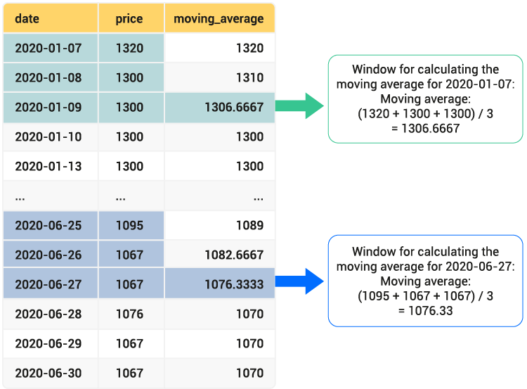
This image shows a practical example of a 3-day moving average calculation. Notice how for each day, the average is calculated using the price of that day and the two previous days.

Just like with other window functions, you can combine these calculations with PARTITION BY to have the calculation restart for each group. For instance, you could find the moving average of sales for each product separately.

Your Turn: Hands-On with Metabase

Time to apply these concepts in Metabase. Let's use the sample database to calculate some running totals and moving averages.

Question 1: What is the cumulative (running) total of revenue over time?

This query will show how total revenue from all orders accumulates chronologically.

1. Navigate to the SQL editor in Metabase.
2. Run the following query:

SELECT
  created_at,
  total,
  SUM(total) OVER (
    ORDER BY created_at
    ROWS BETWEEN UNBOUNDED PRECEDING AND CURRENT ROW
  ) AS running_revenue
FROM orders
ORDER BY created_at;

Look at the running_revenue column. You'll see it increase with each order, as each order's total is added to the sum of all previous orders.

Question 2: What is the 5-order moving average of the order total?

This query will help smooth out the order values to see the recent trend in the average order size.

1. Use the SQL editor to run this query:

SELECT
  created_at,
  total,
  AVG(total) OVER (
    ORDER BY created_at
    ROWS BETWEEN 4 PRECEDING AND CURRENT ROW
  ) AS five_order_moving_avg
FROM orders
ORDER BY created_at;

Here, ROWS BETWEEN 4 PRECEDING AND CURRENT ROW defines a window of 5 orders (the current one + the four before it). For the first four rows of the result set, the average will be calculated over fewer than 5 rows, as there aren't 4 preceding rows yet. This is the correct behavior.

Question 3: What is the running total of revenue for each product category?

This is a classic "Top N per group" style analysis. We want the running total to reset for each product category. This requires PARTITION BY.

1. Run this query in the SQL editor:

SELECT
  p.category,
  o.created_at,
  o.total,
  SUM(total) OVER (
    PARTITION BY p.category
    ORDER BY o.created_at
    ROWS BETWEEN UNBOUNDED PRECEDING AND CURRENT ROW
  ) AS running_category_revenue
FROM orders AS o
JOIN products AS p ON o.product_id = p.id
ORDER BY p.category, o.created_at;

In the results, notice how the running_category_revenue accumulates within each category ("Doohickey", "Gadget", etc.) and then resets to start again when the category changes.

Conclusion

In this lesson, you've added a crucial piece to your analytical SQL skillset: the window frame clause. You now understand how to move beyond simple rankings and offsets to perform sophisticated aggregations like running totals and moving averages. This capability is fundamental to time-series analysis and performance tracking.

Key Takeaways:

• Aggregate Window Functions: Functions like SUM(), AVG(), and COUNT() can be used over a window to produce a value for each row.
• The Window Frame: The frame clause (ROWS BETWEEN ...) gives you explicit control over which rows are included in a calculation for the current row.
• Running Totals: Calculated by defining a frame that extends from the beginning of a partition to the current row (ROWS BETWEEN UNBOUNDED PRECEDING AND CURRENT ROW).
• Moving Averages: Calculated over a sliding window of a fixed size (ROWS BETWEEN N PRECEDING AND CURRENT ROW). This is excellent for trend analysis.
• PARTITION BY: As before, this clause allows you to apply these calculations independently to different groups within your data.

Now that you can calculate sophisticated metrics, the next logical step is to present them effectively. In our next lesson, we will transition from calculation to communication, diving into the principles of data visualization and how to select the appropriate chart types to tell a clear and compelling story with your data.