Singular Value Decomposition and Eigenvalues

Welcome to the second module of our course. In the previous lesson, we concluded our geometric tour of linear algebra by introducing matrix norms, which measure the "size" of a linear transformation. We saw a tantalizing preview of the singular value decomposition (SVD), noting that a matrix's largest singular value, $σ_{m a x}$ , corresponds to its spectral norm—the maximum "stretching factor" it can apply to a vector.

In this lesson, we will formally derive the Singular Value Decomposition. We'll move beyond the geometric intuition and construct the SVD from first principles for any $m \times n$ matrix $A$ . The central goal is to prove that any matrix can be factored into a product of a rotation, a scaling, and another rotation, and to establish the profound connection between a matrix's singular values and the eigenvalues of the related symmetric matrices $A^{T} A$ and $A A^{T}$ .

The Goal: A Universal Decomposition

The eigendecomposition you are familiar with, $A = X Λ X^{- 1}$ , is incredibly powerful, but it has its limitations. It only applies to square matrices, and a well-behaved eigenbasis $X$ isn't always guaranteed. For symmetric matrices, however, the situation is perfect: the decomposition becomes $A = Q Λ Q^{T}$ , where $Q$ is an orthogonal matrix representing a pure rotation. This cleanly separates the transformation's geometry into a rotation ( $Q^{T}$ ), an axis-aligned scaling ( $Λ$ ), and a rotation back ( $Q$ ).

What if we could achieve a similarly clean, geometric decomposition for any matrix, even rectangular ones? This is the core problem that SVD solves. The following reading outlines this motivation and the strategy we will use to solve it.

Deriving SVD from First Principles: An Intuitive Guide

This article provides an intuitive, step-by-step derivation of the SVD. We'll start with the sections that frame the problem and outline the clever strategy for solving it.

Please read the sections titled "The Problem to Solve" and "The Strategy". The key insight is that even if A isn't symmetric, we can always construct symmetric matrices from it—namely, A^TA and AA^T—and leverage their "superpowers".

Deriving the SVD from $A^{T} A$

The strategy is to find a special orthonormal basis for the input space (the row space) and a special orthonormal basis for the output space (the column space) such that the matrix $A$ maps basis vectors from the first set to scaled versions of the basis vectors in the second set.

Let $A$ be an $m \times n$ matrix. We are looking for three matrices, $U$ , $Σ$ , and $V$ , such that $A = U Σ V^{T}$ , where:

$V$ is an $n \times n$ orthogonal matrix whose columns ${v_{i}}$ form an orthonormal basis for the input space $R^{n}$ .
$U$ is an $m \times m$ orthogonal matrix whose columns ${u_{i}}$ form an orthonormal basis for the output space $R^{m}$ .
$Σ$ is an $m \times n$ diagonal matrix containing non-negative "stretching factors" or singular values, $σ_{i}$ .

The core relationship we seek is $A v_{i} = σ_{i} u_{i}$ . Let's see how we can construct these components.

Finding the input basis V and singular values $Σ$ :
The key lies in the symmetric, positive semi-definite matrix $S = A^{T} A$ . Since $S$ is symmetric, it has a full set of orthonormal eigenvectors. Let's call them $v_{1}, v_{2}, \dots, v_{n}$ , which will form the columns of our matrix $V$ . The corresponding eigenvalues $λ_{i}$ are all non-negative.
$(A^{T} A) v_{i} = λ_{i} v_{i}$
Now, let's examine the length of the transformed vectors $A v_{i}$ .
$∥ A v_{i} ∥^{2} = (A v_{i})^{T} (A v_{i}) = v_{i}^{T} A^{T} A v_{i} = v_{i}^{T} (λ_{i} v_{i}) = λ_{i} ∥ v_{i} ∥^{2} = λ_{i}$
This is a remarkable result. The squared length of the transformed vector $A v_{i}$ is simply the corresponding eigenvalue $λ_{i}$ . This naturally leads us to define the singular values $σ_{i}$ as the square roots of these eigenvalues:
$σ_{i} = λ_{i} = ∥ A v_{i} ∥$
Finding the output basis U:
We have the input vectors $v_{i}$ and the scaling factors $σ_{i}$ . All that's left is to define the output vectors $u_{i}$ . The relationship $∥ A v_{i} ∥ = σ_{i}$ suggests a natural definition for the $u_{i}$ . For all singular values $σ_{i} > 0$ , we define $u_{i}$ as the normalized output vector:
$u_{i} = \frac{1}{σ _{i}} A v_{i}$
By definition, these vectors $u_{i}$ are unit vectors. But are they orthogonal? Let's check. For $i \neq = j$ :
$u_{i}^{T} u_{j} = (\frac{1}{σ _{i}} A v_{i})^{T} (\frac{1}{σ _{j}} A v_{j}) = \frac{1}{σ _{i} σ _{j}} v_{i}^{T} (A^{T} A) v_{j} = \frac{1}{σ _{i} σ _{j}} v_{i}^{T} (λ_{j} v_{j}) = \frac{λ _{j}}{σ _{i} σ _{j}} (v_{i}^{T} v_{j})$
Since the eigenvectors $v_{i}$ of the symmetric matrix $A^{T} A$ are orthogonal, $v_{i}^{T} v_{j} = 0$ for $i \neq = j$ . Therefore, $u_{i}^{T} u_{j} = 0$ . The set of vectors ${u_{i}}$ is indeed orthonormal.

We have now successfully constructed the components. The relation $u_{i} = \frac{1}{σ _{i}} A v_{i}$ can be rearranged to $A v_{i} = σ_{i} u_{i}$ . If we write this for all vectors in matrix form, we get $A V = U Σ$ , which gives our final result by multiplying by $V^{T}$ :

A = U Σ V^{T}

The following reading walks through this exact derivation in a narrative style.

Deriving SVD from First Principles: An Intuitive Guide

Now let's see the full derivation laid out. This section puts the pieces from our strategy into a formal argument.

Read the text starting from the formal derivation. Pay close attention to how the orthogonality of V is used to show the orthogonality of the resulting vectors AV, which then leads to the definition of U.

The Role of $A A^{T}$

We built the SVD by analyzing $A^{T} A$ . What happens if we analyze $A A^{T}$ instead? Professor Gilbert Strang offers a particularly elegant perspective that starts with the decomposition $A = U Σ V^{T}$ and examines $A^{T} A$ and $A A^{T}$ to see what they reveal about the components.

Singular Value Decomposition (the SVD)

In this classic MIT OpenCourseWare video, Gilbert Strang derives the SVD's relationship to both AᵀA and AAᵀ.

Watch the following two segments: Analyzing AᵀA: Here, Strang computes A^TA from A=U\Sigma V^T. The result is A^TA = V(\Sigma^T\Sigma)V^T. This is precisely the eigendecomposition of A^TA, confirming that V is the matrix of eigenvectors and the eigenvalues are \lambda_i = \sigma_i^2. Analyzing AAᵀ: He then does the same for AA^T, yielding AA^T = U(\Sigma\Sigma^T)U^T. This shows that U must be the matrix of eigenvectors for AA^T, and its non-zero eigenvalues are also \sigma_i^2.

This confirms a symmetric and beautiful relationship. The two matrices $A^{T} A$ and $A A^{T}$ , while potentially of different sizes, are intimately linked. They share the same non-zero eigenvalues ( $σ_{i}^{2}$ ), and their respective eigenvector matrices are none other than the $V$ and $U$ from the SVD of $A$ .

The following reading provides one final confirmation of this fact.

Deriving SVD from First Principles: An Intuitive Guide

This short section provides the algebraic proof that U is the eigenbasis of AAᵀ, solidifying the connection.

Please read the section titled "U is an Eigenbasis of AAᵀ". This completes the puzzle, showing how U, V, and Σ tie everything together.

Summary of the SVD

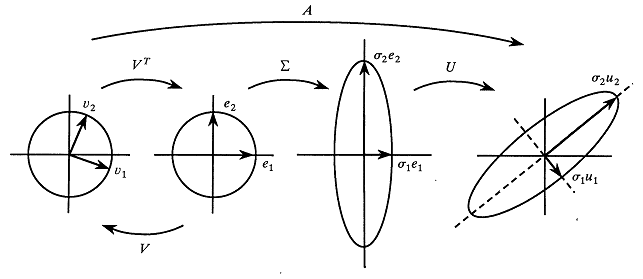
Let's consolidate what we have derived. For any $m \times n$ matrix $A$ of rank $r$ , its Singular Value Decomposition is $A = U Σ V^{T}$ .

The SVD of an $m \times n$ matrix A is composed of an $m \times m$ orthogonal matrix U, an $m \times n$ diagonal matrix Σ containing singular values, and the transpose of an $n \times n$ orthogonal matrix V.

The geometric interpretation of this decomposition is a sequence of three operations:

Rotation ( $V^{T}$ ): An input vector $x$ is rotated by $V^{T}$ without changing its length. The new coordinates are in the basis of the right singular vectors ( $v_{i}$ ).
Scaling ( $Σ$ ): The rotated vector is stretched along each of the new axes by the corresponding singular values $σ_{i}$ .
Rotation ( $U$ ): The scaled vector is rotated by $U$ to its final position in the output space.

The SVD decomposes the action of matrix A on a unit circle into three steps: a rotation (Vᵀ), an axis-aligned scaling by singular values $\sigma_1, \sigma_2$ (Σ), and a final rotation (U). The result is an ellipse whose semi-axes are defined by the singular values and oriented by the left singular vectors.

Conclusion

In this lesson, we have formally derived the Singular Value Decomposition, one of the most fundamental and versatile tools in linear algebra.

Key Takeaways:

Any $m \times n$ matrix $A$ can be factored as $A = U Σ V^{T}$ , where $U$ and $V$ are orthogonal matrices and $Σ$ is a diagonal matrix of non-negative singular values.
The right singular vectors (columns of $V$ ) are the orthonormal eigenvectors of the symmetric matrix $A^{T} A$ .
The left singular vectors (columns of $U$ ) are the orthonormal eigenvectors of the symmetric matrix $A A^{T}$ .
The non-zero singular values ( $σ_{1}, \dots, σ_{r}$ ) are the square roots of the non-zero eigenvalues of both $A^{T} A$ and $A A^{T}$ .

So far, we have focused on the existence and derivation of the SVD. In the next lesson, we will put this powerful tool to work, using it to analyze fundamental properties of a matrix, such as its rank, condition number, and the geometry of its four fundamental subspaces.

Recommended resources

The Goal: A Universal Decomposition

Deriving the SVD from ATA

The Role of AAT

Summary of the SVD

Conclusion

Deriving the SVD from $A^{T} A$

The Role of $A A^{T}$