PCA: Variance Maximization and the Spectral Theorem

1. The Duality of PCA: Maximizing Variance vs. Minimizing Error

At its core, PCA seeks a lower-dimensional projection of a dataset that preserves as much "information" as possible. But what does it mean to preserve information? There are two equivalent ways to frame this goal, which turn out to be two sides of the same coin.

1. Maximizing Variance: We can project the data onto a new, lower-dimensional subspace such that the variance of the projected data is maximized. The intuition here is that directions with high variance are the most informative, while directions with low or zero variance are redundant or noisy.

2. Minimizing Reconstruction Error: We can project the data and then reconstruct it back into the original space. The goal is to find a projection that minimizes the squared distance between the original data points and their reconstructions.

The following image illustrates this duality. The gray line represents a potential principal component. Projecting the blue data points onto this line maximizes their spread (variance) along the line, while simultaneously minimizing the length of the red lines (the projection or reconstruction error).

We can see why these two objectives are equivalent through a simple geometric argument based on the Pythagorean theorem. Consider a single mean-centered data point $\mathbf{x}$ and its projection onto the direction defined by a unit vector $\mathbf{u}$.

A single data point $\mathbf{x}$ is projected onto the line defined by the unit vector $\mathbf{u}$. The projection is ${\mathbf{x}}^{\prime }$, the reconstruction error is $\mathbf{r}$, and the squared length of the projection is $z^2$.

The original vector $\mathbf{x}$ forms the hypotenuse of a right-angled triangle. The other two sides are the projection vector ${\mathbf{x}}^{\prime }$ and the error vector $\mathbf{r}=\mathbf{x}-{\mathbf{x}}^{\prime }$. The squared length of the projection is $z^2=({\mathbf{x}}^T\mathbf{u}{)}^2$. By the Pythagorean theorem:

Since the original data points $\mathbf{x}$ are fixed, $\Vert \mathbf{x}{\Vert }^2$ is a constant for each point. Therefore, maximizing the projected variance (which we'll see is a sum of $z^2$ terms) is equivalent to minimizing the sum of squared reconstruction errors ($\Vert \mathbf{r}{\Vert }^2$).

For a more formal walkthrough of this equivalence, the following reading is excellent.

While both perspectives are valid, the variance-maximization framework leads to a more direct and elegant derivation, which we will now pursue.

2. Deriving PCA: An Eigenvalue Problem

Let's formalize the problem of finding the direction of maximum variance. Assume we have a dataset represented by a matrix $X$ of size $N\times P$, where $N$ is the number of data points and $P$ is the number of features. We'll assume the data has been mean-centered, meaning the mean of each feature column has been subtracted, so the dataset's centroid is at the origin.

Our goal is to find the direction, represented by a unit vector $\mathbf{u}$ of size $P\times 1$, that maximizes the variance of the data when projected onto it.

The projection of a single data point ${\mathbf{x}}_i^T$ (a row vector) onto the direction $\mathbf{u}$ is a scalar value ${\mathbf{x}}_i^T\mathbf{u}$. The variance of these projected points is:

Since we are maximizing this quantity, the constant factor $\frac{1}{N-1}$ can be ignored. Our objective function becomes:

This expression can be rewritten in a more convenient matrix form. The summation is the squared norm of the projected data vector $X\mathbf{u}$:

The matrix $X^{T}X$ is closely related to the sample covariance matrix, $C=\frac{1}{N-1}{X}^{T}X$. So, maximizing ${\mathbf{u}}^T{X}^{T}X\mathbf{u}$ is equivalent to maximizing ${\mathbf{u}}^{T}C\mathbf{u}$. This quantity is a quadratic form, which, as we saw in the previous lesson, describes how the transformation $C$ stretches space. We are looking for the direction $\mathbf{u}$ where the stretch is greatest.

Our optimization problem is now:

This is a constrained optimization problem that can be solved using Lagrange multipliers. The Lagrangian is:

Taking the gradient with respect to $\mathbf{u}$ and setting it to zero gives:

This is the fundamental eigenvector equation for the covariance matrix $C$. It shows that the optimal direction $\mathbf{u}$ must be an eigenvector of the covariance matrix.

But which one? To find out, let's substitute this result back into our objective function:

This is a crucial result. The variance of the data projected onto an eigenvector $\mathbf{u}$ is simply the corresponding eigenvalue $\lambda$. To maximize the variance, we must choose the eigenvector corresponding to the largest eigenvalue.

This eigenvector is the first principal component (${\mathbf{u}}_1$). The second principal component (${\mathbf{u}}_2$) is the direction that maximizes variance while being orthogonal to ${\mathbf{u}}_1$, and so on. The Spectral Theorem, which we covered last lesson, guarantees that for a symmetric matrix like $C$, all its eigenvectors are mutually orthogonal. Thus, the principal components form an ordered, orthogonal basis, with each component corresponding to an eigenvector of the covariance matrix, ordered from the largest eigenvalue to the smallest.

The following resource provides an elegant and detailed walkthrough of this derivation.

3. Interpreting the Components

We have now formally derived the main result of PCA:

• The principal components are the orthonormal eigenvectors of the data's covariance matrix $C$.
• The variance of the data projected onto each principal component ${\mathbf{u}}_i$ is the corresponding eigenvalue ${\lambda }_i$.

This provides a clear recipe for finding and interpreting the components. The eigenvectors tell us the directions of greatest variance, and the eigenvalues tell us the magnitude of that variance.

By sorting the eigenvalues in descending order, ${\lambda }_1\ge {\lambda }_2\ge \cdots \ge {\lambda }_P\ge 0$, we get a natural ranking of the principal components in terms of their importance. The total variance in the data is given by the trace of the covariance matrix, which is also equal to the sum of its eigenvalues:

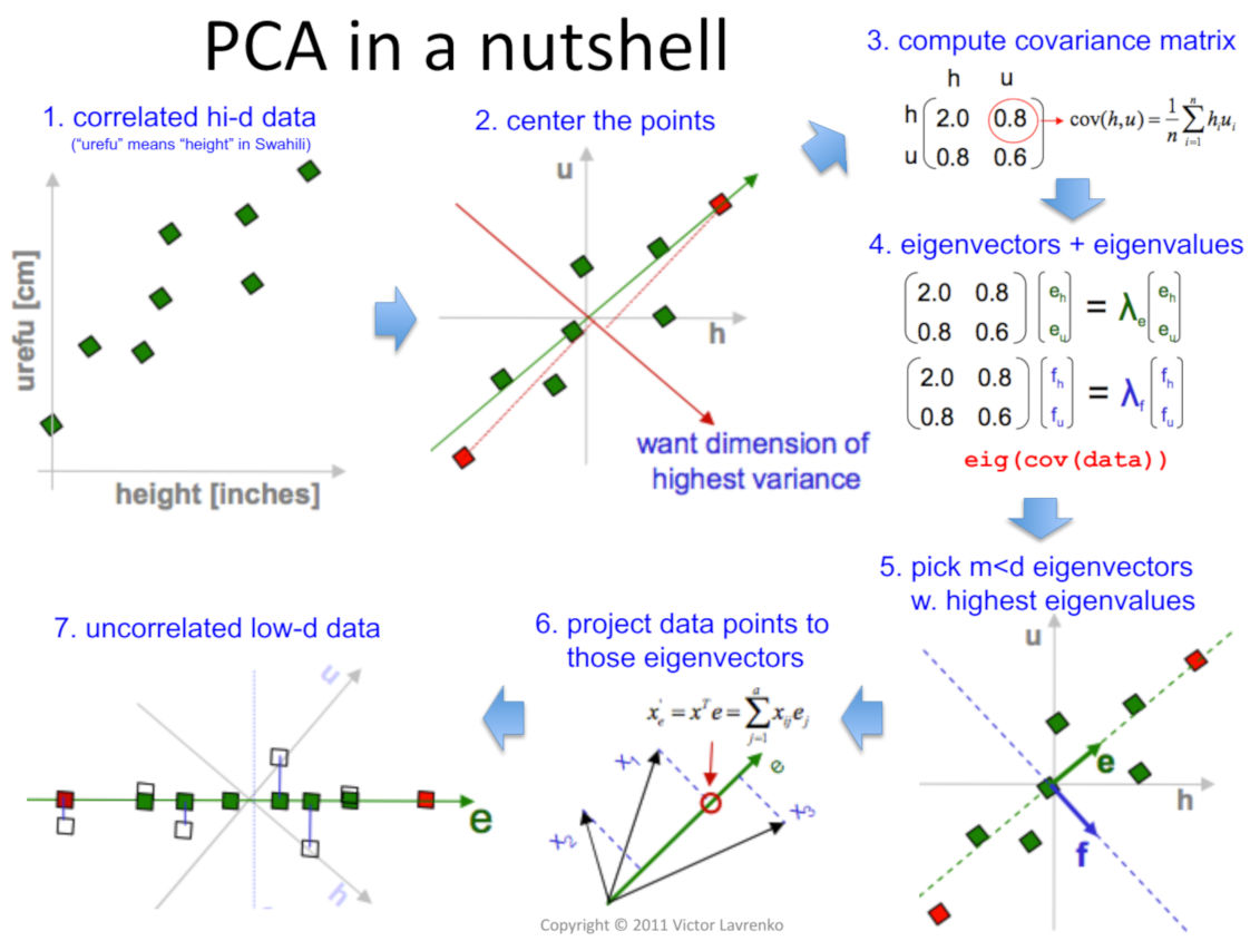
The fraction of total variance "explained" by the $k$-th principal component is simply ${\lambda }_k/{\sum }_i{\lambda }_i$. This allows us to perform dimensionality reduction in a principled way: we can keep the first $K$ principal components that capture a desired percentage (e.g., 95%) of the total variance, and discard the rest. The data transformed into this new basis, $Z=XV$, where the columns of $V$ are the top $K$ eigenvectors, will have uncorrelated features whose variances are the eigenvalues.

The following visual summary captures the entire process, from a correlated dataset to the final, uncorrelated principal components.

To solidify your understanding of these final steps, please continue with the same article.

Conclusion

In this lesson, we have formally derived Principal Component Analysis from the ground up, connecting the intuitive goal of preserving information to a concrete mathematical procedure.

Key Takeaways:

• PCA aims to find a lower-dimensional representation of data by either maximizing the variance of the projected data or, equivalently, minimizing the reconstruction error.
• Formulating PCA as a variance-maximization problem leads to the optimization problem ${\max }_{\mathbf{u}}{\mathbf{u}}^{T}C\mathbf{u}$ subject to ${\mathbf{u}}^T\mathbf{u}=1$, where $C$ is the covariance matrix.
• The solution to this problem reveals that the principal components are the eigenvectors of the covariance matrix.
• The variance of the data along the direction of each principal component is given by its corresponding eigenvalue.
• This provides a principled method for dimensionality reduction: by ranking components by their eigenvalues, we can retain the most significant dimensions of variation and discard the least significant ones.

This lesson concludes our module on matrix decompositions. We have seen how SVD and eigendecomposition are not just abstract mathematical tools, but powerful lenses for analyzing the structure of data, models, and loss landscapes. Having established this geometric foundation, we will now pivot to the calculus of optimization. Our next module begins by laying the groundwork for automatic differentiation, starting with the fundamentals of vector and matrix calculus.