Spectral Theorem for Symmetric Matrices in Statistical Applications

1. The Spectral Theorem: A Guarantee of Order

The Spectral Theorem provides a definitive statement about the structure of real symmetric matrices. In essence, it says that any transformation represented by a symmetric matrix can be understood as a simple sequence of a rotation, a scaling along orthogonal axes, and a rotation back.

Formally, the Spectral Theorem states that if $S$ is a real symmetric matrix ($S=S^T$), then:

1. All eigenvalues of $S$ are real numbers.
2. Eigenvectors corresponding to distinct eigenvalues are orthogonal.
3. $S$ is always orthogonally diagonalizable. This means there exists an orthogonal matrix $Q$ and a diagonal matrix $\Lambda$ such that: $$S=Q\Lambda Q^T$$ Here, the columns of $Q$ are an orthonormal set of eigenvectors of $S$, and the diagonal entries of $\Lambda$ are the corresponding eigenvalues.

This decomposition, $S=Q\Lambda Q^T$, is not just an algebraic curiosity; it is a profound geometric statement. The Visual Kernel channel has a fantastic video that brings this decomposition to life.

The video shows that the seemingly complex transformation of a symmetric matrix $S$ becomes simple when viewed in its natural coordinate system—the eigenbasis. For a deeper look at the formal proof, which is quite elegant, you can refer to the appendix in the PCA tutorial we will use shortly.

With this powerful theorem in hand, let's see what it reveals when applied to important matrices in machine learning.

2. Application 1: The Covariance Matrix

The covariance matrix is arguably the most common symmetric matrix in data science. It quantifies the shape and orientation of a cloud of data points. For a dataset with $m$ features, the $m\times m$ covariance matrix $\Sigma$ has the variance of each feature on its diagonal and the covariance between pairs of features on its off-diagonals.

The following video provides a quick, visual introduction to what a covariance matrix represents.

The video correctly points out that the goal is to find the axes along which the data varies the most. This is precisely what applying the Spectral Theorem to the covariance matrix achieves. Since $\Sigma$ is symmetric, we can write:

This decomposition has a specific and powerful interpretation:

• The columns of $Q$ are the principal components of the data. They form an orthonormal basis where the first vector points in the direction of maximum variance, the second points in the direction of maximum variance in the subspace orthogonal to the first, and so on.
• The diagonal entries of $\Lambda$ are the eigenvalues ${\lambda }_i$, which represent the variance of the data projected onto each corresponding principal component.

By re-expressing our data in the basis of $Q$, we diagonalize the covariance matrix, meaning the new features (the principal components) are uncorrelated. This is the essence of Principal Component Analysis (PCA).

Let's delve deeper into this derivation.

3. Application 2: The Kernel Matrix

Kernel methods, such as Support Vector Machines (SVMs) and Gaussian Processes, use a kernel function $k(x,x^{\prime })$ to measure similarity between data points. For a dataset $\{x_1,\dots ,x_n\}$, this gives rise to the $n\times n$ kernel matrix $K$ (also called the Gram matrix), where $K_{ij}=k(x_i,x_j)$.

Since $k(x,x^{\prime })=k(x^{\prime },x)$, the kernel matrix $K$ is always symmetric. For most useful kernels (e.g., Gaussian/RBF, polynomial), $K$ is also positive semi-definite, meaning all its eigenvalues are non-negative (${\lambda }_i\ge 0$).

Applying the Spectral Theorem to $K$, we get $K=Q\Lambda Q^T$. What does this tell us?

This decomposition is central to an area known as kernel PCA. While standard PCA finds principal components in the input space, kernel PCA finds principal components in the high-dimensional feature space implicitly defined by the kernel. The eigenvectors of the kernel matrix $K$ (the columns of $Q$) provide the principal directions of variation of the data in that feature space.

A fascinating aspect, especially relevant to your goal of understanding generative models, is the relationship between the spectrum of the empirical kernel matrix and the spectrum of the underlying data-generating process.

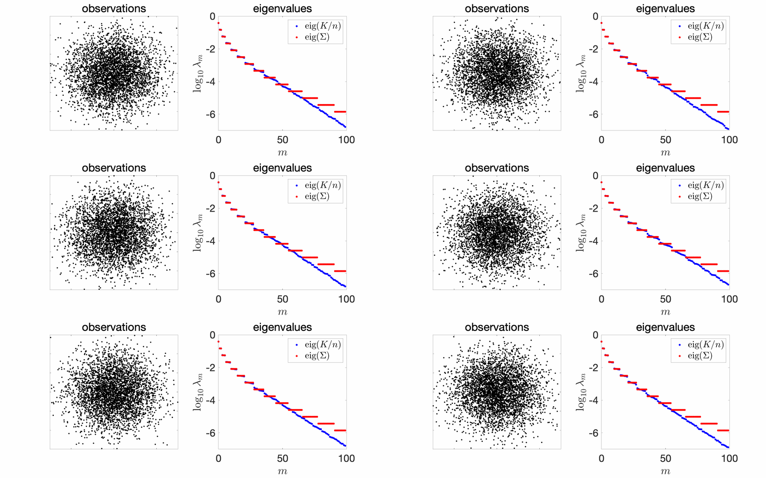
This image illustrates a deep result from statistical learning theory: the eigenvalues of the kernel matrix computed from data samples converge to the eigenvalues of the true, underlying covariance operator. In essence, the eigendecomposition of the kernel matrix allows us to empirically estimate the spectral properties of the (often unknown) process that generated our data.

4. Application 3: The Fisher Information Matrix

Our final application, the Fisher Information Matrix (FIM), takes us to the heart of information geometry and advanced optimization methods in deep learning.

The FIM, denoted $F$, measures how much information a random variable $y$ carries about the parameters $\theta$ of the model $p(y|\theta )$ that generates it. It is defined as the covariance of the score function (${\nabla }_{\theta }\log p(y|\theta )$):

By construction, $F$ is symmetric and positive semi-definite. Therefore, the Spectral Theorem applies: $F=Q\Lambda Q^T$.

This decomposition provides a way to understand the geometry of the parameter space itself.

• The eigenvectors of $F$ (columns of $Q$) define the principal axes of "information sensitivity". An eigenvector with a large eigenvalue points in a direction in parameter space where a small change to the parameters $\theta$ causes a large change in the model's output distribution $p(y|\theta )$.
• The eigenvalues of $F$ (diagonal of $\Lambda$) quantify this sensitivity. Large eigenvalues correspond to highly sensitive or "informative" parameter directions.

This has a direct connection to the Hessian we studied last lesson. Under certain conditions, the FIM is equal to the expected value of the Hessian of the negative log-likelihood. So, the FIM can be seen as a measure of the average curvature of the loss landscape.

This insight is the foundation for Natural Gradient Descent (NGD). While standard gradient descent follows the steepest descent direction in the Euclidean geometry of the parameter space, NGD follows the steepest descent in the information geometry defined by the FIM. The update rule is:

Using the spectral decomposition $F^{-1}=Q{\Lambda }^{-1}{Q}^T$, we can see that NGD effectively rescales the gradient. It takes smaller steps in sensitive directions (large eigenvalues of $F$) and larger steps in less sensitive directions (small eigenvalues of $F$). It adapts the learning process to the intrinsic geometry of the statistical manifold, often leading to faster convergence than standard gradient descent.

Conclusion

In this lesson, we formalized the properties of symmetric matrices through the lens of the Spectral Theorem and saw how its application yields profound insights across different areas of machine learning.

Key Takeaways:

• The Spectral Theorem guarantees that any real symmetric matrix $S$ can be decomposed into $Q\Lambda Q^T$, where $Q$ is an orthogonal matrix of eigenvectors and $\Lambda$ is a diagonal matrix of real eigenvalues. This is geometrically equivalent to a rotation, an axis-aligned scaling, and a rotation back.
• For a covariance matrix, this decomposition yields the principal components of the data and their corresponding variances, forming the basis of PCA.
• For a kernel matrix, the decomposition reveals the principal axes of variation in a high-dimensional feature space, and its spectrum can approximate that of the underlying data-generating process.
• For the Fisher Information Matrix, the decomposition identifies the directions of highest sensitivity in the model's parameter space, providing the geometric foundation for advanced optimizers like natural gradient descent.

Having seen how the spectral theorem applies to covariance matrices, we are now perfectly positioned for our next lesson, where we will formally derive Principal Component Analysis (PCA) from the spectral theorem and interpret its components as the directions that maximize the variance of our data.