Understanding Entropy and Divergence

Hello! In our last lesson, we derived the reparameterization trick, a clever method for backpropagating through stochastic nodes in a computational graph. This gave us a low-variance way to compute gradients for the part of a VAE's objective that involves reconstructing the input. However, that's only half the story. The full VAE objective, the Evidence Lower Bound (ELBO), involves another critical component: a term that regularizes the latent space.

This regularization term is almost always a Kullback-Leibler (KL) divergence. To fully grasp how VAEs work, and indeed how many generative models and classification problems are framed, we need to build a solid, intuitive understanding of the core concepts from information theory. This lesson is dedicated to defining and exploring three of the most important measures: entropy, cross-entropy, and KL divergence. We will not only formalize them but also compute them for both simple discrete cases and for the Gaussian distributions that are central to models like VAEs and diffusion models.

1. From Surprise to Entropy: Measuring Uncertainty

The most intuitive way to approach information theory is by starting with the concept of "surprise." An event that is very unlikely to happen is more surprising when it occurs than a very common event. Information theory quantifies this intuition.

A mathematically convenient way to define surprise, or self-information, is with a logarithm. We want surprise to be additive for independent events (the surprise of two independent dice rolls should be the sum of their individual surprises), while probabilities multiply. The logarithm neatly converts products to sums.

The surprisal $s (x)$ of an outcome $x$ with probability $p (x)$ is defined as:

s (x) = - lo g p (x)

The negative sign ensures that surprise is non-negative, as $p (x)$ is between 0 and 1. As $p (x) \to 0$ , $s (x) \to \infty$ . As $p (x) \to 1$ , $s (x) \to 0$ .

While surprisal applies to a single outcome, entropy characterizes the distribution as a whole. It is the average or expected surprise over all possible outcomes.

For a random variable $X$ with probability distribution $P$ , the entropy $H (P)$ or $H (X)$ is:

H (X) = E_{x \sim P} [s (x)] = E_{x \sim P} [- lo g p (x)]

Specifically:

For a discrete variable with probability mass function $p (x_{i})$ : $H (X) = - i \sum p (x_{i}) lo g p (x_{i})$
For a continuous variable with probability density function $p (x)$ , this is called differential entropy: $H (X) = - \int p (x) lo g p (x) d x$

The following video provides an excellent visual and conceptual foundation for these ideas, building from the ground up.

The Key Equation Behind Probability

This video from Artem Kirsanov provides a wonderfully intuitive derivation of entropy starting from the idea of surprise.

Watch the first part, which formalizes the notion of surprise and how it relates to probability: Surprise and Log-Probability. Continue with the next segment, which defines entropy as the average surprise and gives a concrete example: From Surprise to Entropy.

Entropy measures the inherent unpredictability or uncertainty in a distribution. A distribution with a single certain outcome has zero entropy. For a discrete distribution with a fixed number of outcomes, a uniform distribution (where all outcomes are equally likely) has the maximum possible entropy.

2. Cross-Entropy and KL Divergence: Measuring the Mismatch

In machine learning, we rarely have access to the true data-generating distribution, which we can call $P$ . Instead, we build a model, let's call it $Q$ , to approximate $P$ . A natural question arises: how much "average surprise" do we experience if we observe events drawn from the true distribution $P$ , but we evaluate their surprise using the probabilities from our model $Q$ ? This measure is the cross-entropy.

Formally, the cross-entropy between $P$ and $Q$ is:

H (P, Q) = E_{x \sim P} [- lo g q (x)]

Notice the key difference from entropy: we are taking an expectation over samples from $P$ , but the logarithm is applied to the probabilities from $Q$ .

Cross-entropy is the foundation for the loss function in nearly all classification tasks. When you use a "cross-entropy loss", you are implicitly minimizing the cross-entropy between the true distribution of labels (e.g., a one-hot vector) and the predicted probabilities from your model.

Now, we can relate these concepts.

The entropy $H (P)$ is the minimum possible average surprise, achieved only if we have a perfect model ( $Q = P$ ).
The cross-entropy $H (P, Q)$ is the average surprise we actually experience using our (likely imperfect) model $Q$ .

The difference between them is the extra surprise, or inefficiency, caused by using an approximate model instead of the true one. This difference is the Kullback-Leibler (KL) divergence.

D_{K L} (P ∥ Q) = H (P, Q) - H (P)

By substituting the definitions and using the properties of logarithms, we get the standard form:

D_{K L} (P ∥ Q) = E_{x \sim P} [- lo g q (x)] - E_{x \sim P} [- lo g p (x)] = E_{x \sim P} [lo g \frac{p ( x )}{q ( x )}]

This relationship, $H (P, Q) = H (P) + D_{K L} (P ∥ Q)$ , is fundamental. It tells us that minimizing the cross-entropy with respect to our model $Q$ is equivalent to minimizing the KL divergence, because $H (P)$ is a constant that doesn't depend on $Q$ .

The following resources provide further intuition and formal definitions for these crucial concepts.

Fantastic KL Divergence and How to (Actually) Compute It

This video by Jia-Bin Huang offers a compact, practical explanation using the analogy of optimal coding.

Watch the first part which quickly recaps surprise and entropy: Surprise and Entropy. Then, watch the explanation of cross-entropy and KL divergence as the "extra bits" needed for a suboptimal code: Cross-Entropy and KL Divergence.

22.11. Information Theory

The D2L.ai book provides concise, formal definitions and discusses the key properties of these measures.

First, review the formal definitions of Entropy for both discrete and continuous cases. Next, read the definition of KL Divergence and its properties. Finally, read the formal definition of Cross-Entropy and note its relationship to the other two measures.

An important property of KL divergence is that it is not symmetric: in general, $D_{K L} (P ∥ Q) \neq = D_{K L} (Q ∥ P)$ . This asymmetry has profound consequences in how different generative models behave, a topic we will explore in a future lesson.

3. Computation for Discrete Distributions

Let's make this concrete with a simple discrete example. Suppose the true distribution for a 3-sided die is $P = [0.5, 0.25, 0.25]$ . Our model believes the die is fair, so $Q = [1/3, 1/3, 1/3]$ . Let's calculate the information-theoretic measures (using log base 2 for "bits").

Entropy of P:
$H (P) = - (0.5 lo g_{2} 0.5 + 0.25 lo g_{2} 0.25 + 0.25 lo g_{2} 0.25) = - (0.5 \cdot (- 1) + 0.25 \cdot (- 2) + 0.25 \cdot (- 2)) = 1.5 bits$
This is the inherent uncertainty of the true distribution.
Cross-Entropy H(P, Q):
$H (P, Q) = - (0.5 lo g_{2} (1/3) + 0.25 lo g_{2} (1/3) + 0.25 lo g_{2} (1/3)) = - lo g_{2} (1/3) = lo g_{2} (3) \approx 1.585 bits$
This is the average number of bits we'd need to encode outcomes from P using a code optimized for Q.
KL Divergence D_KL(P || Q):
$D_{K L} (P ∥ Q) = H (P, Q) - H (P) \approx 1.585 - 1.5 = 0.085 bits$
This is the "cost" or "wasted information" from using the uniform model Q to describe the data from P.

This plot shows entropy and cross-entropy for a simpler case, the Bernoulli distribution (a two-sided die or coin). The purple curve shows the entropy $H(q)$ of a coin with probability of heads $q$, which is maximized at $q=0.5$ (a fair coin). The other curves show the cross-entropy between a true distribution (e.g., fair, $p=0.5$) and a model distribution with parameter $q$. Notice cross-entropy is minimized when the model matches the true distribution ($q=p$).

4. Derivation for Gaussian Distributions

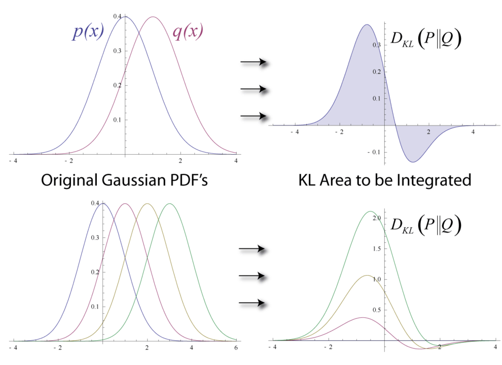
For VAEs, the most important application is calculating the KL divergence between two Gaussian distributions. The encoder network typically outputs the parameters of an approximate posterior distribution $q (z ∣ x) = N (μ_{q}, σ_{q}^{2})$ , and we want to measure its divergence from a simple prior, usually a standard normal $p (z) = N (0, 1)$ .

Let's derive the general formula for the KL divergence between two univariate Gaussians, $p = N (μ_{1}, σ_{1}^{2})$ and $q = N (μ_{2}, σ_{2}^{2})$ .

The definition is:

D_{K L} (p ∥ q) = \int p (x) lo g \frac{p ( x )}{q ( x )} d x = \int p (x) (lo g p (x) - lo g q (x)) d x

This is equivalent to $E_{x \sim p} [lo g p (x) - lo g q (x)]$ .

The log-probability for a Gaussian $N (μ, σ^{2})$ is:

lo g N (x; μ, σ^{2}) = - \frac{1}{2} lo g (2 π σ^{2}) - \frac{( x - μ ) ^{2}}{2 σ ^{2}}

Let's calculate the expectation of each log-term under $p (x) = N (μ_{1}, σ_{1}^{2})$ :

$E_{x \sim p} [lo g p (x)]$ :
$E_{x \sim p} [- \frac{1}{2} lo g (2 π σ_{1}^{2}) - \frac{( x - μ _{1} ) ^{2}}{2 σ _{1}^{2}}] = - \frac{1}{2} lo g (2 π σ_{1}^{2}) - \frac{1}{2 σ _{1}^{2}} E_{x \sim p} [(x - μ_{1})^{2}]$
Since $E_{x \sim p} [(x - μ_{1})^{2}] = σ_{1}^{2}$ by definition of variance, this simplifies to:
$E_{x \sim p} [lo g p (x)] = - \frac{1}{2} lo g (2 π σ_{1}^{2}) - \frac{1}{2} = - \frac{1}{2} (lo g (2 π e σ_{1}^{2}))$
This is the negative of the differential entropy of the Gaussian.
$E_{x \sim p} [lo g q (x)]$ :
$E_{x \sim p} [- \frac{1}{2} lo g (2 π σ_{2}^{2}) - \frac{( x - μ _{2} ) ^{2}}{2 σ _{2}^{2}}] = - \frac{1}{2} lo g (2 π σ_{2}^{2}) - \frac{1}{2 σ _{2}^{2}} E_{x \sim p} [(x - μ_{2})^{2}]$
For the expectation term, we can expand it: $E [(x - μ_{2})^{2}] = E [(x - μ_{1} + μ_{1} - μ_{2})^{2}] = E [(x - μ_{1})^{2} + 2 (x - μ_{1}) (μ_{1} - μ_{2}) + (μ_{1} - μ_{2})^{2}]$ .
Using linearity of expectation, and that $E [x - μ_{1}] = 0$ , this becomes $σ_{1}^{2} + (μ_{1} - μ_{2})^{2}$ .
Substituting back:
$E_{x \sim p} [lo g q (x)] = - \frac{1}{2} lo g (2 π σ_{2}^{2}) - \frac{σ _{1}^{2} + ( μ _{1} - μ _{2} ) ^{2}}{2 σ _{2}^{2}}$

Finally, we compute $D_{K L} (p ∥ q) = E_{x \sim p} [lo g p (x)] - E_{x \sim p} [lo g q (x)]$ :

D_{K L} (N (μ_{1}, σ_{1}^{2}) ∥ N (μ_{2}, σ_{2}^{2})) = (- \frac{1}{2} lo g (2 π σ_{1}^{2}) - \frac{1}{2}) - (- \frac{1}{2} lo g (2 π σ_{2}^{2}) - \frac{σ _{1}^{2} + ( μ _{1} - μ _{2} ) ^{2}}{2 σ _{2}^{2}}) = \frac{1}{2} (lo g \frac{σ _{2}^{2}}{σ _{1}^{2}} - 1 + \frac{σ _{1}^{2} + ( μ _{1} - μ _{2} ) ^{2}}{σ _{2}^{2}}) = lo g \frac{σ _{2}}{σ _{1}} + \frac{σ _{1}^{2} + ( μ _{1} - μ _{2} ) ^{2}}{2 σ _{2}^{2}} - \frac{1}{2}

This closed-form expression is what you will implement in PyTorch for the VAE. It allows you to compute the KL divergence term of the loss analytically, without needing Monte Carlo estimation.

This image visualizes the KL divergence between two Gaussian distributions. The top-left shows two distributions, $p(x)$ and $q(x)$. The top-right shows the function $p(x) \log(p(x)/q(x))$, whose integral gives the KL divergence. The bottom plot shows that as the distributions become more dissimilar, the KL divergence (the area under the curve) increases.

Conclusion

Today, we've journeyed through the foundational concepts of information theory that are indispensable for modern machine learning. You now have both an intuitive and a formal understanding of these key measures.

Key Takeaways:

Entropy $H (P)$ measures the inherent uncertainty or "average surprise" of a probability distribution.
Cross-Entropy $H (P, Q)$ measures the average surprise when observing data from a true distribution $P$ but using a model $Q$ to calculate probabilities. It's a standard loss function in classification.
Kullback-Leibler (KL) Divergence $D_{K L} (P ∥ Q)$ measures the "extra surprise" or inefficiency from using model $Q$ instead of the true distribution $P$ . It quantifies the mismatch between two distributions.
The relationship $H (P, Q) = H (P) + D_{K L} (P ∥ Q)$ shows why minimizing cross-entropy is equivalent to minimizing KL divergence for model optimization.
For the crucial case of two Gaussian distributions, the KL divergence can be calculated analytically, a key component for training VAEs.

You now possess all the mathematical components needed to understand the objective function of a Variational Autoencoder. In our next lesson, we will put everything together by deriving the Evidence Lower Bound (ELBO), and you will see exactly how the KL divergence we derived today serves as the essential regularization term that structures the latent space.

Recommended resources

1. From Surprise to Entropy: Measuring Uncertainty

2. Cross-Entropy and KL Divergence: Measuring the Mismatch

3. Computation for Discrete Distributions

4. Derivation for Gaussian Distributions

Conclusion