Pathwise Gradient Estimator for Stochastic Operations

1. The Problem: Differentiating Through a Stochastic Node

Let's formalize the problem. In a model like a VAE, an encoder network with parameters $\varphi$ outputs the parameters of a distribution for a latent variable $z$, for example, the mean ${\mu }_{\varphi }(x)$ and variance ${\sigma }_{\varphi }^2(x)$ of a Gaussian $q_{\varphi }(z|x)$. We then draw a sample $z\sim q_{\varphi }(z|x)$. This sample $z$ is fed into a decoder network to produce an output.

To train the encoder, we need to backpropagate a loss signal through the decoder, through the sampled $z$, and ultimately to the parameters $\varphi$. The sampling step, however, breaks this chain. The act of drawing a random sample is a stochastic process, not a deterministic function of the distribution's parameters. Automatic differentiation frameworks like PyTorch cannot compute a gradient through this random operation.

The following resource clearly articulates this roadblock.

This "broken graph" is visualized in the left panel of the diagram below. The blue circular node for $z$ represents a random or stochastic node, through which gradients cannot flow.

2. An Alternative Path: The Score Function Estimator

Before introducing the reparameterization trick, it's useful to know about an alternative method for handling this problem: the score function estimator, also known as the log-derivative trick or REINFORCE algorithm (common in reinforcement learning).

Without going into a full derivation, it relies on the identity ${\nabla }_{\varphi }{q}_{\varphi }(z)=q_{\varphi }(z){\nabla }_{\varphi }\log q_{\varphi }(z)$. This allows us to rewrite the gradient of the expectation as another expectation:

This resulting expectation can be approximated with Monte Carlo sampling. Notice that we no longer need to differentiate $f(z)$. The gradient is computed on the log-probability of the distribution itself.

While this approach works and is quite general (it doesn't require $f$ to be differentiable), it is notorious for suffering from high variance. The Monte Carlo estimate of this gradient can be extremely noisy from one batch of samples to the next, making training unstable and slow. The intuition is that the estimator's value can be dominated by rare samples $z$ for which $f(z)$ is large, leading to erratic updates.

The following resource provides an excellent, intuitive explanation of this high-variance issue.

3. The Reparameterization Trick: Creating a Differentiable Path

The reparameterization trick offers a more elegant and, crucially, lower-variance solution for many common distributions. The core idea is to re-express the random variable $z$ in a way that isolates the stochasticity from the parameters $\varphi$.

Instead of sampling $z$ directly from $q_{\varphi }(z|x)$, we express it as a deterministic and differentiable function $g_{\varphi }(\cdot )$ that takes two inputs:

1. The parameters from our encoder (e.g., ${\mu }_{\varphi }(x),{\sigma }_{\varphi }(x)$).
2. An auxiliary noise variable $ϵ$, sampled from a simple, fixed distribution $p(ϵ)$ that does not depend on $\varphi$ (e.g., a standard normal $\mathcal{N}(0,I)$).

So, we define $z=g_{\varphi }(ϵ,x)$ where $ϵ\sim p(ϵ)$.

The most common application of this is with Gaussian latent variables. If our encoder specifies $q_{\varphi }(z|x)=\mathcal{N}({\mu }_{\varphi }(x),{\sigma }_{\varphi }^2(x)I)$, we can reparameterize the sampling of $z$ as:

Here, $\odot$ denotes element-wise multiplication. The random variable $z$ still has the desired distribution $\mathcal{N}({\mu }_{\varphi }(x),{\sigma }_{\varphi }^2(x)I)$, but we have created a deterministic computational path from ${\mu }_{\varphi }$ and ${\sigma }_{\varphi }$ to $z$, as shown in the right panel of the Reparameterization Trick Computational Graph diagram. The stochasticity is now "injected" via $ϵ$, which is external to the gradient path.

The following video provides a clear visual and conceptual walkthrough of this transformation.

4. Derivation of the Pathwise Gradient Estimator

With this re-framing, we can now derive the gradient estimator. Our goal is to compute ${\nabla }_{\varphi }{\mathbb{E}}_{z\sim q_{\varphi }(z|x)}[f(z)]$.

1. Rewrite the expectation: Using the reparameterization $z=g_{\varphi }(ϵ,x)$ with $ϵ\sim p(ϵ)$, we change the distribution over which we are taking the expectation:

   $${\mathbb{E}}_{z\sim q_{\varphi }(z|x)}[f(z)]={\mathbb{E}}_{ϵ\sim p(ϵ)}[f(g_{\varphi }(ϵ,x))]$$

2. Move the gradient inside: Now, we take the gradient with respect to $\varphi$. Since the distribution $p(ϵ)$ does not depend on $\varphi$, and assuming $f$ and $g_{\varphi }$ are differentiable, we can move the gradient operator inside the expectation. This is the crucial step that was not possible before.

   $${\nabla }_{\varphi }{\mathbb{E}}_{ϵ\sim p(ϵ)}[f(g_{\varphi }(ϵ,x))]={\mathbb{E}}_{ϵ\sim p(ϵ)}[{\nabla }_{\varphi }f(g_{\varphi }(ϵ,x))]$$

3. Apply Monte Carlo estimation: The expression inside the final expectation, ${\nabla }_{\varphi }f(g_{\varphi }(ϵ,x))$, can be computed using standard backpropagation (i.e., the chain rule) for a given sample of $ϵ$. We can then approximate the full expectation with a simple Monte Carlo estimate, often using just a single sample $L=1$ of $ϵ$ for each data point $x$ in a mini-batch.

   $${\nabla }_{\varphi }{\mathbb{E}}_{z\sim q_{\varphi }(z|x)}[f(z)]\approx \frac{1}{L}\sum _{l=1}^L{\nabla }_{\varphi }f(g_{\varphi }({ϵ}^{(l)},x))\text{where }{ϵ}^{(l)}\sim p(ϵ)$$

This final expression is the pathwise gradient estimator. The following resource provides the formal derivation and discusses its benefits.

5. Practical Impact: Variance Reduction

The primary reason for the reparameterization trick's success is that it yields a gradient estimator with significantly lower variance than the score function estimator. This leads to much more stable and faster convergence during training.

We can see this empirically. The image below shows the results of a simple optimization problem: finding the parameters $(\mu ,\sigma )$ of a normal distribution to minimize ${\mathbb{E}}_{X\sim \mathcal{N}(\mu ,{\sigma }^2)}[X^2]$. The clear answer is $\mu =0,\sigma =0$. The plots compare the convergence behavior when using the reparameterization trick versus the score function estimator.

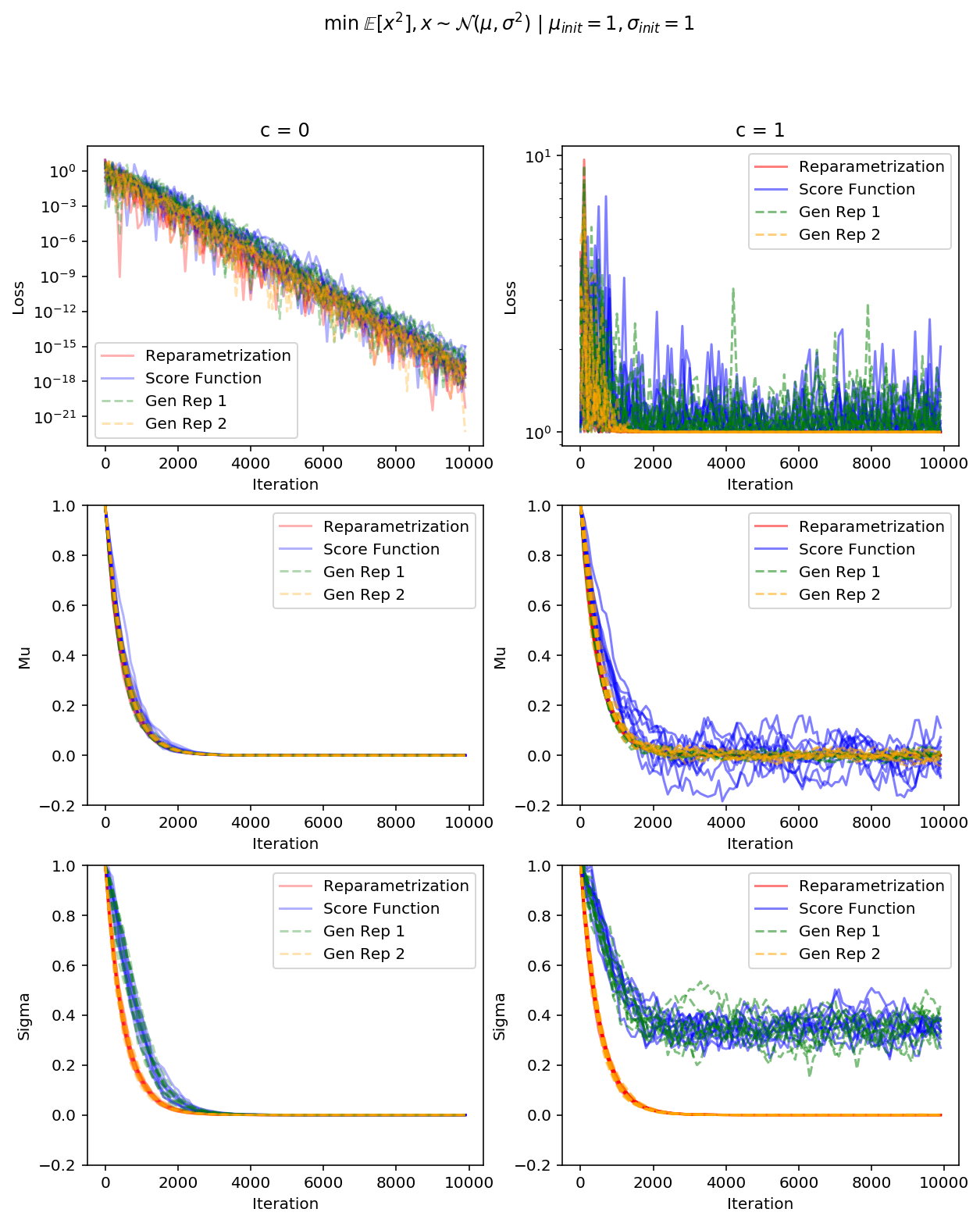
As you can see, the pathwise gradients (labeled "Reparameterization") provide a smooth and direct path to the optimal parameters. The score function gradients are so noisy that the parameters bounce around wildly, and the loss decreases much more erratically. For complex, high-dimensional models, this difference in variance is often the difference between a model that trains successfully and one that fails to converge at all.

Conclusion

In this lesson, we have moved from simply estimating expectations to optimizing them. You have derived a critical tool for training stochastic deep learning models.

Key Takeaways:

• Differentiating an expectation ${\mathbb{E}}_{z\sim q_{\varphi }}[f(z)]$ with respect to the distribution's parameters $\varphi$ is challenging because standard backpropagation cannot flow through a stochastic sampling node.
• The score function estimator provides a general solution but often suffers from high-variance gradients, leading to unstable training.
• The reparameterization trick (or pathwise estimator) solves this for many continuous distributions by reformulating the random variable $z$ as a deterministic, differentiable function of its parameters $\varphi$ and an independent noise source $ϵ$.
• This reformulation allows the gradient operator ${\nabla }_{\varphi }$ to be moved inside the expectation, yielding an estimator that can be computed with standard automatic differentiation.
• The primary advantage of the pathwise estimator is its significantly lower variance, which enables stable and efficient training of models like VAEs.

You now understand the core mechanism that makes training VAEs and other similar generative models feasible. This trick allows us to get a low-variance gradient for the reconstruction term of the Evidence Lower Bound (ELBO). In our next lesson, we will dissect the other key component of the ELBO: the Kullback-Leibler (KL) divergence, which acts as a regularizer on the latent space.