Bernoulli, Categorical, and Cross-Entropy for Discrete Outcomes

Welcome to our new lesson. In our previous discussion, we explored how the laws of total expectation and variance allow us to decompose and analyze uncertainty in hierarchical systems. This provided a powerful framework for reasoning about the structure of complex models.

Today, we shift our focus from the structure of uncertainty to the fundamental building blocks used to model it. Your objective is to model discrete outcomes using Bernoulli and Categorical distributions and connect them to the cross-entropy loss. We will establish a direct and crucial link between the statistical principle of Maximum Likelihood Estimation (MLE) and the loss functions you routinely use to train classification models in PyTorch. This lesson will make the probabilistic underpinnings of your practical work explicit.

1. Modeling Binary Outcomes: The Bernoulli Distribution

The simplest case of a discrete outcome is a binary choice: yes/no, heads/tails, 0/1. The probability distribution that governs such an event is the Bernoulli distribution.

10-315 Notes Maximum Likelihood Estimation

These lecture notes from Carnegie Mellon University provide a clear, formal definition of the key distributions we'll use. We'll start with the Bernoulli distribution.

Please read section 1.1 Bernoulli. Focus on the definition, the parameter \phi, and the probability mass function (p.m.f.).

As the notes describe, a Bernoulli random variable $Y$ takes the value 1 with probability $ϕ$ and 0 with probability $1 - ϕ$ . We can write its probability mass function in a single, compact expression:

p (y ∣ ϕ) = ϕ^{y} (1 - ϕ)^{1 - y} for y \in {0, 1}

This elegant form is a notational workhorse. When $y = 1$ , the expression becomes $ϕ^{1} (1 - ϕ)^{0} = ϕ$ . When $y = 0$ , it becomes $ϕ^{0} (1 - ϕ)^{1} = 1 - ϕ$ . You will see this pattern appear constantly in derivations involving log-likelihoods.

2. From Probability to Loss: The MLE Connection

How do we connect this abstract probability distribution to training a neural network? The bridge is the principle of Maximum Likelihood Estimation (MLE). MLE states that we should choose the model parameters that maximize the probability (the likelihood) of observing our training data.

For a binary classification task, our model (e.g., a logistic regression or a neural net with a final sigmoid activation) outputs a value $y^$ between 0 and 1. We can interpret this output as our estimate of the Bernoulli parameter $ϕ$ . The ground truth label is $y \in {0, 1}$ .

If we assume our data points are independent and identically distributed (i.i.d.), the total likelihood of the dataset is the product of the individual likelihoods. It's more convenient to work with the log-likelihood, which turns this product into a sum:

ℓ (ϕ; D) = lo g i = 1 \prod N p (y^{(i)} ∣ ϕ) = i = 1 \sum N lo g p (y^{(i)} ∣ ϕ)

Substituting our compact Bernoulli p.m.f.:

ℓ (ϕ; D) = i = 1 \sum N lo g (ϕ^{y^{(i)}} (1 - ϕ)^{1 - y^{(i)}}) = i = 1 \sum N [y^{(i)} lo g ϕ + (1 - y^{(i)}) lo g (1 - ϕ)]

Maximizing the log-likelihood is equivalent to minimizing the negative log-likelihood. The negative log-likelihood (NLL) for a single data point is:

NLL (ϕ, y) = - [y lo g ϕ + (1 - y) lo g (1 - ϕ)]

If we replace our model's prediction $y^$ for the parameter $ϕ$ , we get precisely the binary cross-entropy loss function used in deep learning. The following reading walks through this derivation in the context of logistic regression.

10-315 Notes Maximum Likelihood Estimation

This section makes the connection between the MLE objective and the loss function explicit.

Please read section 4.2.1 Binary logistic regression. Pay close attention to how the log-likelihood function (Eq. 121) is transformed into the final optimization objective (Eq. 126), which you'll recognize as the standard binary cross-entropy loss.

This is a profound connection: minimizing cross-entropy is not an arbitrary choice but is equivalent to finding the maximum likelihood parameters for a model that assumes the data is generated from a Bernoulli distribution.

3. Modeling Multi-Class Outcomes: The Categorical Distribution

When we have more than two discrete outcomes, we generalize from the Bernoulli to the Categorical distribution. This is the probabilistic foundation for multi-class classification.

10-315 Notes Maximum Likelihood Estimation

Now let's look at the generalization of the Bernoulli to K classes.

Read section 1.2 Categorical. Note how it's parameterized by a vector \phi and how the random variable Y is represented as a one-hot vector.

For a Categorical distribution with $K$ classes, the random variable is a one-hot vector $y$ of length $K$ . The distribution is parameterized by a probability vector $ϕ = [ϕ_{1}, \dots, ϕ_{K}]$ where $\sum_{k} ϕ_{k} = 1$ . The probability of observing class $k$ (i.e., $y_{k} = 1$ ) is $ϕ_{k}$ .

Similar to the Bernoulli case, we can write a compact p.m.f. using the one-hot encoding of the outcome $y$ :

p (y ∣ ϕ) = k = 1 \prod K ϕ_{k}^{y_{k}}

Since $y$ is a one-hot vector, only the term for the true class will have a non-zero exponent, effectively selecting the correct probability $ϕ_{k}$ .

Following the same MLE logic, the negative log-likelihood for a single data point is:

NLL (ϕ, y) = - lo g k = 1 \prod K ϕ_{k}^{y_{k}} = - k = 1 \sum K y_{k} lo g ϕ_{k}

In a neural network for multi-class classification, the final linear layer produces scores (logits), which are passed through a softmax function to produce the probability vector $y^$ that we use as our estimate for $ϕ$ . The ground truth is the one-hot label vector $y$ . The resulting loss function is the categorical cross-entropy loss.

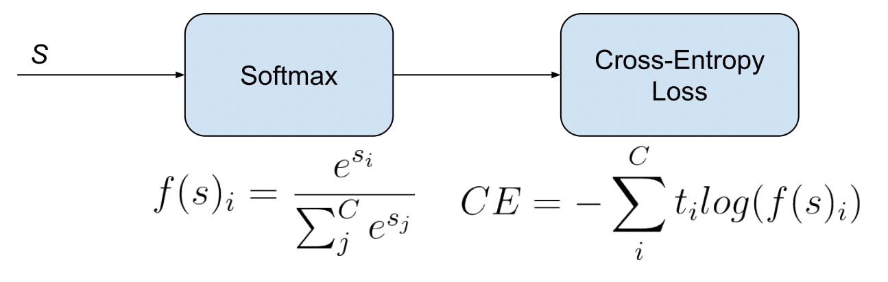
This diagram illustrates the standard pipeline for multi-class classification. The input scores $S$ (logits) are transformed by the Softmax function into a probability distribution $f(s)$. This distribution is then compared against the true target distribution $t$ (a one-hot vector) using the Cross-Entropy loss formula to compute the final loss value.

The derivation is analogous to the binary case, as shown in the next reading.

10-315 Notes Maximum Likelihood Estimation

This section completes the picture by extending the MLE-loss connection to the multi-class setting.

Read section 4.2.2 Multi-class logistic regression. Follow the derivation from the likelihood (Eq. 131) to the log-likelihood (Eq. 135) and finally to the optimization objective (Eq. 140). This final form is exactly the categorical cross-entropy loss.

4. NLL vs. Cross-Entropy: Two Sides of the Same Coin

In deep learning frameworks like PyTorch, you'll see the classification loss referred to as CrossEntropyLoss, while in probabilistic modeling literature, the objective is to minimize the NegativeLogLikelihood. As we've just derived, for discrete outcomes modeled by Bernoulli/Categorical distributions, these are mathematically identical.

Why the two names?

Negative Log-Likelihood describes the objective from the perspective of statistical estimation (MLE).
Cross-Entropy describes the same mathematical formula, but from the perspective of information theory. It measures the "distance" between the true data distribution (a one-hot vector representing certainty) and the model's predicted probability distribution.

The following video provides an excellent, intuitive explanation of this equivalence.

What is the difference between negative log likelihood and cross entropy? (in neural networks)

This video directly addresses the common confusion between Negative Log-Likelihood and Cross-Entropy loss in the context of training neural networks.

Watch the entire video. The key parts are: The derivation of the Negative Log-Likelihood for a multi-class problem. Notice how it arrives at the same formula we derived: -\sum_k y_k \log \hat{y}_k. The comparison to the definition of Cross-Entropy, where the presenter shows that if you treat the one-hot ground truth as one distribution (p) and the model's softmax output as the other (q), the formula is identical.

This equivalence solidifies the idea that training a classification network is a form of probabilistic modeling. Every time you use cross-entropy loss, you are implicitly assuming a Bernoulli or Categorical likelihood for your data and performing maximum likelihood estimation.

Conclusion

In this lesson, we have forged a critical link between fundamental probability theory and the everyday practice of deep learning. We've seen how the simple, elegant models for discrete outcomes—the Bernoulli and Categorical distributions—provide the theoretical justification for using cross-entropy loss in classification tasks.

Key Takeaways:

The Bernoulli distribution models a binary outcome and is parameterized by a single probability $ϕ$ .
The Categorical distribution models an outcome from $K$ discrete classes and is parameterized by a probability vector $ϕ$ .
The principle of Maximum Likelihood Estimation (MLE) provides a framework for fitting these distributions to data.
Minimizing the negative log-likelihood (NLL) under a Bernoulli or Categorical assumption is mathematically equivalent to minimizing the binary or categorical cross-entropy loss, respectively.
Therefore, training a classifier with cross-entropy loss is a form of principled probabilistic inference.

In our next lesson, we will extend this approach to continuous variables. We will explore the Gaussian distribution, which is not only the foundation for regression tasks (where it connects to Mean Squared Error loss) but is also a cornerstone of the advanced generative models you plan to implement, including VAEs and Diffusion Models.

Recommended resources

1. Modeling Binary Outcomes: The Bernoulli Distribution

2. From Probability to Loss: The MLE Connection

3. Modeling Multi-Class Outcomes: The Categorical Distribution

4. NLL vs. Cross-Entropy: Two Sides of the Same Coin

Conclusion