Gaussian Models in Machine Learning

1. The Multivariate Gaussian Distribution

The most important probability distribution for continuous variables is the Gaussian, or normal, distribution. While you're familiar with its univariate "bell curve" form, in deep learning we almost always deal with high-dimensional vectors. This requires the multivariate Gaussian distribution.

A $d$-dimensional multivariate Gaussian is completely specified by two parameters:

• A mean vector $\mu \in {\mathbb{R}}^d$, which defines its center.
• A covariance matrix $\Sigma \in {\mathbb{R}}^{d\times d}$, which must be symmetric and positive semi-definite. This matrix defines the shape and orientation of the distribution.

The following reading from a University of Toronto lecture provides a formal introduction to the multivariate Gaussian and its parameters.

As you saw in the notes, the probability density function (PDF) is given by:

Let's briefly dissect this expression, as its components are central to many deep learning concepts:

• The term $(x-\mu {)}^T{\Sigma }^{-1}(x-\mu )$ is a quadratic form known as the squared Mahalanobis distance. It measures the distance from a point $x$ to the mean $\mu$, accounting for the covariance structure. The level sets of the PDF (the contour lines in the 2D plots) are ellipsoids defined by keeping this distance constant.
• The eigenvectors of $\Sigma$ define the principal axes of these ellipsoids, and the corresponding eigenvalues determine the variance along those axes.
• The term $|\Sigma {|}^{1/2}$ in the denominator is a normalization constant. As the determinant $|\Sigma |$ corresponds to the product of eigenvalues, it reflects the "volume" of the distribution. A larger volume (more spread out) leads to a smaller peak density.

2. Connection 1: Regression and Mean Squared Error

Our first practical connection is to linear regression. In the previous lesson, we saw that minimizing cross-entropy loss is equivalent to performing Maximum Likelihood Estimation with a Categorical distribution. We can now show that minimizing Mean Squared Error (MSE) is equivalent to performing MLE with a Gaussian distribution.

Let's assume our target variable $t$ is generated by a linear function of inputs $x$ plus some random noise $ϵ$:

If we model this noise as being drawn from a zero-mean Gaussian distribution, $ϵ\sim \mathcal{N}(0,{\sigma }^2)$, then the conditional probability of the target $t$ given the input $x$ is also Gaussian:

This states that our model's prediction, $y=w^{T}x$, is the mean of the Gaussian distribution from which the true target is drawn.

Given a dataset of $N$ i.i.d. examples, the log-likelihood is the sum of the individual log-probabilities. Maximizing this log-likelihood will give us the most likely parameter $w$.

This derivation reveals a profound insight: the widespread use of MSE for regression tasks is not arbitrary. It is the direct consequence of assuming that the data is generated with Gaussian-distributed errors. This probabilistic interpretation also provides a framework for more advanced techniques, such as viewing L2 regularization as MAP inference with a Gaussian prior on the weights, as shown in the subsequent slides of the same resource.

3. Connection 2: VAEs and the Reparameterization Trick

The Gaussian distribution is also fundamental to many generative models, including the Variational Autoencoder (VAE) you plan to implement.

In a VAE, the encoder network does not map an input $x$ to a single latent point $z$. Instead, it maps $x$ to the parameters of a probability distribution in the latent space, typically a Gaussian. That is, the encoder outputs a mean vector ${\mu }_{\theta }(x)$ and a covariance matrix ${\Sigma }_{\theta }(x)$ (often simplified to a diagonal matrix). A latent code $z$ is then sampled from this distribution: $z\sim \mathcal{N}({\mu }_{\theta }(x),{\Sigma }_{\theta }(x))$.

This sampling step introduces a major challenge: it is a stochastic, non-differentiable operation. How can we backpropagate the reconstruction error from the decoder back to the encoder's parameters $\theta$, if there's a random sampling node in between?

The solution is the reparameterization trick, which relies on a key property of Gaussians. We can generate a sample from any Gaussian $\mathcal{N}(\mu ,\Sigma )$ by taking a sample $ϵ$ from a standard normal distribution $\mathcal{N}(0,I)$ and applying an affine transformation:

where $L$ is a matrix such that $L{L}^T=\Sigma$ (for instance, the Cholesky decomposition of $\Sigma$). If $\Sigma$ is diagonal, $\Sigma =\text{diag}({\sigma }_1^2,\dots ,{\sigma }_d^2)$, this simplifies to $z=\mu +\sigma \odot ϵ$, where $\sigma$ is the vector of standard deviations and $\odot$ is element-wise multiplication.

The reading below formalizes this "shift and scale" property.

By reframing the sampling process this way, we cleverly sidestep the non-differentiable part. The stochasticity is now externalized into the $ϵ$ term, which is a fixed input and does not depend on any model parameters. The path from the encoder's parameters ($\mu ,\sigma$) to the latent code $z$ is now a deterministic, differentiable function.

The following video provides a detailed walkthrough of this entire concept.

4. Connection 3: Diffusion Noise

Finally, the Gaussian distribution is the engine behind Denoising Diffusion Probabilistic Models (DDPMs), another key paper you aim to implement. The entire principle of diffusion models rests on a carefully defined process of incrementally adding Gaussian noise.

The forward process of a DDPM starts with a clean data point $x_0$ (e.g., an image) and gradually corrupts it over $T$ timesteps. At each step $t$, the new state $x_t$ is sampled from a Gaussian distribution whose mean is a slightly contracted version of the previous state $x_{t-1}$:

Here, ${\beta }_t$ is a small, pre-defined constant that controls the amount of noise added at step $t$. By repeating this process, we form a Markov chain that transforms any complex data distribution into pure Gaussian noise by time $T$.

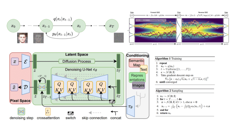
A critical property of this process, which stems from the fact that a sum of Gaussian variables is also Gaussian, is that we can compute the distribution of $x_t$ given the original $x_0$ in a single step, without iterating through all intermediate steps. This makes training a network to reverse this process—to denoise $x_t$—tractable. The Gaussian distribution's analytical tractability is what makes the entire DDPM framework computationally feasible.

Conclusion

In this lesson, we have explored the central role of the Gaussian distribution in modeling continuous data for deep learning. We have seen that it is not just a statistical curiosity but the theoretical foundation for many standard practices and advanced models.

Key Takeaways:

• The Multivariate Gaussian distribution is defined by a mean vector $\mu$ and a covariance matrix $\Sigma$, which dictates its ellipsoidal geometry.
• Minimizing Mean Squared Error (MSE) in regression is equivalent to performing Maximum Likelihood Estimation under the assumption of Gaussian noise.
• The reparameterization trick, enabled by the affine transformation property of Gaussians, allows for gradient-based training of models with stochastic latent variables, like VAEs.
• The forward process in diffusion models is constructed as a Markov chain that systematically injects Gaussian noise, a process whose properties are essential for training the reverse, generative model.

We have used the affine transformation property of Gaussians today to understand sampling and reparameterization. In our next lesson, we will delve deeper, using this same property along with the change of variables formula to formally derive the multivariate Gaussian PDF from first principles. This will complete your understanding of where this fundamental density function comes from.